1. Confined Aquifer Test - Oude Korendijk

This example is taken from Kruseman et al. 1970

Step 1: Loading packages

import matplotlib.pyplot as plt
import numpy as np
import pandas as pd

import ttim as ttm

plt.rcParams["figure.figsize"] = (5, 3)  # default figure size

Introduction and Conceptual Model

TTim is a semi-analytical model of transient groundwater flow systems (Bakker, 2013). It applies the Laplace-transform analytic element method to solve for groundwater flow in a variety of hydrogeological features. One of the many applications of TTim is the analysis of aquifer tests. In this series of Jupyter Notebooks, we demonstrate the capabilities to model and calibrate aquifer tests in different hydrogeological conditions.

In this example, we will use the pumping test data from Oude Korendijk (Kruseman et al. 1970) to demonstrate how TTim can be used to model and analyze pumping tests. Furthermore, we reproduce the work of Yang (2020) and compare the performance of TTim with other transient well hydraulics software AQTESOLV (Duffield, 2007) and MLU (Carlson and Randall, 2012).

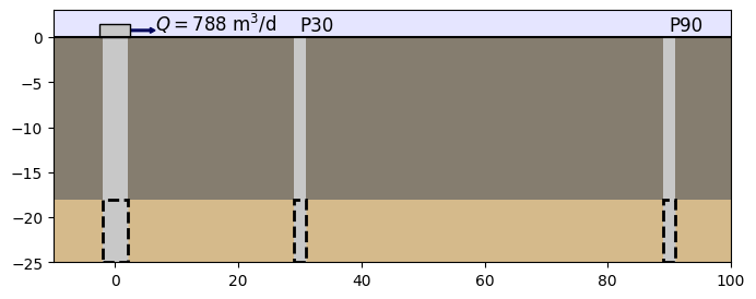
Oude Korendijk is a polder area south of Rotterdam, the Netherlands. The stratigraphy can be summarised by:

• the presence in the first 18 m depth of an impermeable layer,

• followed by a 7 m succession of coarse gravel and sands, which are considered as the aquifer layer,

• and finally, a layer of fine sands and clayey sediments that are deemed impermeable.

The well screens the whole thickness of the aquifer. Drawdowns were taken from piezometers installed 30 and 90 m away from the well. Pumping at the well has been taken with a constant discharge of 788 m3/d for almost 14 hours.

The conceptual model of the area is a single layer confined aquifer located at 18 m below surface and 7 m thickness. At \(t=0\), the pumping starts at a constant discharge of 788 m3/d and drawdowns are recorded at two piezometers, 30 and 90 meters away, respectively. The figure below summarises the conceptualization of the problem

Show code cell source

Hide code cell source

import matplotlib.pyplot as plt

##Now printing the conceptual model figure:

fig = plt.figure(figsize=(8, 3))
ax = fig.add_subplot(1, 1, 1)
# sky
sky = plt.Rectangle((-10, 0), width=110, height=3, fc="b", zorder=0, alpha=0.1)
ax.add_patch(sky)

# Aquifer:
ground = plt.Rectangle(
    (-10, -25),
    width=110,
    height=25,
    fc=np.array([209, 179, 127]) / 255,
    zorder=0,
    alpha=0.9,
)
ax.add_patch(ground)

# Confining bed:
confining_unit = plt.Rectangle(
    (-10, -18),
    width=110,
    height=18,
    fc=np.array([100, 100, 100]) / 255,
    zorder=0,
    alpha=0.7,
)
ax.add_patch(confining_unit)
well = plt.Rectangle(
    (-2, -25), width=4, height=25, fc=np.array([200, 200, 200]) / 255, zorder=1
)
ax.add_patch(well)

# Wellhead
wellhead = plt.Rectangle(
    (-2.5, 0), width=5, height=1.5, fc=np.array([200, 200, 200]) / 255, zorder=2, ec="k"
)
ax.add_patch(wellhead)

# Screen for the well:
screen = plt.Rectangle(
    (-2, -25),
    width=4,
    height=7,
    fc=np.array([200, 200, 200]) / 255,
    alpha=1,
    zorder=2,
    ec="k",
    ls="--",
)
screen.set_linewidth(2)
ax.add_patch(screen)
pumping_arrow = plt.Arrow(x=2.5, y=0.75, dx=4, dy=0, color="#00035b")
ax.add_patch(pumping_arrow)
ax.text(x=6.5, y=0.75, s=r"$ Q = 788$ m$^3$/d", fontsize="large")
# Piezometers
piez1 = plt.Rectangle(
    (29, -25), width=2, height=25, fc=np.array([200, 200, 200]) / 255, zorder=1
)
piez2 = plt.Rectangle(
    (89, -25), width=2, height=25, fc=np.array([200, 200, 200]) / 255, zorder=1
)
screen_piez_1 = plt.Rectangle(
    (29, -25),
    width=2,
    height=7,
    fc=np.array([200, 200, 200]) / 255,
    alpha=1,
    zorder=2,
    ec="k",
    ls="--",
)
screen_piez_1.set_linewidth(2)
screen_piez_2 = plt.Rectangle(
    (89, -25),
    width=2,
    height=7,
    fc=np.array([200, 200, 200]) / 255,
    alpha=1,
    zorder=2,
    ec="k",
    ls="--",
)
screen_piez_2.set_linewidth(2)
ax.add_patch(piez1)
ax.add_patch(piez2)
ax.add_patch(screen_piez_1)
ax.add_patch(screen_piez_2)
# last line
line = plt.Line2D(xdata=[-10, 100], ydata=[0, 0], color="k")
ax.add_line(line)
ax.text(x=30, y=0.75, s="P30", fontsize="large")
ax.text(x=90, y=0.75, s="P90", fontsize="large")
ax.set_xlim([-10, 100])
ax.set_ylim([-25, 3]);

Step 2: Setting basic parameters for the model

H = 7  # aquifer thickness in meters, m
zt = -18  # top boundary of aquifer, m
zb = zt - H  # bottom boundary of aquifer, m
Q = 788  # constant discharge, m3/d

Step 3: Creating a TTim conceptual model

In this example, we are using the ModelMaq model to conceptualize our aquifer. ModelMaq defines the aquifer system as a stacked vertical sequence of aquifers and leaky layers (aquifer-leaky layer, aquifer-leaky layer, etc). Aquifers are conceptualized as having no vertical resistance (Dupuit approximation), with constant hydraulic conductivity and storage. Aquitard layers are approximated as having only vertical flow. They are characterized by the parameter resistance to vertical flow and by having no storage.

In the model construction, we have to set the parameters for each layer (which consists of an aquifer layer and an aquitard layer).

For our one-layer model we have to set:

• The hydraulic conductivity: kaq this is a list/array with a float element for every aquifer, for example: [kaq0,kaq1]. We can also set a float value, in this case, the same kaq is assumed for every layer.

• The top and bottom of each aquifer: z defined by a list/array [zt0,zb0,zt1,zb1,...], where the inputs are a sequence of top and bottoms of the aquifer layers.

• The specific storage: Saq. The input is a list/array with a float element for every aquifer, for example: [Saq0, Saq1]. We can also set a float value. In this case, the same Saq is assumed for every layer.

• The minimum time for which TTim solve the groundwater flow: tmin, a float.

• And the maximum time: tmax, float.

Optional parameters:

• TTim automatically assumes the topboundary is confined (topboundary = 'conf'). If we assign: topboundary = 'semi' This means that we assume the layer on top of the uppermost aquifer is a leaky layer, and we must also characterize it. Thus, even though we have only one aquifer, we have to set an additional element to the z array, which is the top of the aquitard formation:

  • For example: z = [0,zt,zb]. 0 is the depth of the aquitard overlying the aquifer, zt and zb are the top and bottom of the aquifer.

  • We would also specify the leaky-layer parameters c and Sll (see below).

• phreatictop: Is a boolean (True/False). If True, the first element in Saq is considered phreatic storage (Specific Yield) and it is not multiplied by the layer thickness. The default value is False in ModelMaq. Generally, this parameter is set to True only in unconfined aquifers.

In case of more than one layer model, or when topboundary = 'semi', we would also have to set the resistance to vertical flow c, and the storage Sll of the aquitard portions. An example of this configuration can be seen in the notebook Confined 4 - Schroth

To represent our pumping well, we will use the Well feature.

Wells, in TTim, are features with specified discharge. The well may be screened in multiple layers. In case the screen is in more than one layer, TTim distributes the discharge across the layers such that the head inside the well is the same in all screened layers. The wellbore storage and skin effect may be taken into account.

The discharge of the well acting on layer \(n\) is computed inside TTim with the expression (Bakker, 2013):

\[ Q_n = 2\pi r_wH_n\frac{h_n-h_w}{c_e} \]

where, \(Q_n\) is the discharge at layer \(n\), which is a positive value for water being pumped, \(r_w\) is the radius of the well, \(H_n\) is the layer thickness, \(h_n\) is the head just outside the well, and \(h_w\) is the head inside the well. \(c_e\) is the entry resistance that can be defined in TTim by the skin resistance of the well (see notebook Confined 2 - Grindley for more details)

For the well we have to set:

• The TTim model: ml where the well is added to

• The x and y location: xw, yw, floats

• The pumping scheme is defined by a list (tsandQ) where each element is a tuple representing a new stress condition with the starting time and the discharge rate, in our case: (0, Q) meaning that pumping begins at t = 0 with pumping rate Q

• The layers where it is screened: layers. This argument can be set as an integer (one layer) or a list/array of integers (multi-screen well).

Optional parameters for the Well object are:

• The well radius: rw, a float, if not specified a value of 0.1 m is assumed.

• the skin resistance of the well: res. If not specified, it is set to 0. An example of setting up the skin resistance is seen in the notebook : Confined 2 - Grindley.

• The radius of the caisson: rc. The radius of the caisson is the parameter used to account for wellbore storage in the simulation. If not specified, this value is set to None and TTim will ignore wellbore storage. TTim considers the wellbore storage by solving the water balance inside the well with the expression (Bakker, 2013):

  \[\pi r_c^2 \frac{dh_w}{dt} = \sum_nQ_n-Q_w \]
  where: \(Q_n\) and \(Q_w\) are the inflows and outflows in the well, \(h_w\) is the head inside the well and \(r_c\) is the radius of the caisson.

# unkonwn parameters: kaq, Saq
ml = ttm.ModelMaq(kaq=60, z=[zt, zb], Saq=1e-4, tmin=1e-5, tmax=1)
w = ttm.Well(ml, xw=0, yw=0, rw=0.2, tsandQ=[(0, Q)], layers=0)

# Here we are setting everything in meters for length and days for time

The last step in our model creation is to “solve” the model:

ml.solve()

self.neq  1
solution complete

Step 4: Load data of two observation wells:

The preferred method of loading data into TTim is to use numpy arrays.

The data is in a text file where the first column is the time data in minutes and the second column is the drawdown in meters

We load the data as a numpy array for each piezometer. We then separate time and drawdown into two different 1d arrays. We also convert time data from minutes to days

# time and drawdown of piezometer 30m away from pumping well
data1 = np.loadtxt("data/piezometer_h30.txt", skiprows=1)
t1 = data1[:, 0] / 60 / 24  # convert min to days
h1 = data1[:, 1]
r1 = 30
# time and drawdown of piezometer 90m away from pumping well
data2 = np.loadtxt("data/piezometer_h90.txt", skiprows=1)
t2 = data2[:, 0] / 60 / 24  # convert min to days
h2 = data2[:, 1]
r2 = 90

Step 5: Calibration

Model Calibration is done in TTim using the Calibrate object. TTim calibrates the parameters by minimizing an objective function using a non-linear least-squares fitting algorithm. The objective function used is the sum of the squares of the residuals calculated as:

\[\sum_n (h_o - h_c)^2\]

,

where \(h_0\) is the observed heads and \(h_c\) is the calculated heads by the model.

and TTim uses lmfit, a python package for non-linear least-squares minimization (Newville et al. 2014), to find the optimal parameters that minimize the residuals.

For the calibration of our groundwater model, we proceed by creating a calibration object with the Calibrate class. The Calibrate object takes the model ml as argument. We then set the parameters we are adjusting:

• Hydraulic conductivity: kaq0 (Hydraulic conductivity of layer 0)

• Specific Storage Saq0 (Specific Storage of layer 0)

with the .set_parameter method.

• .set_parameter takes two arguments:

• name is the parameter name, a string, where the letters define the parameter. The possible values are “kaq”, “Saq” or ‘c’, and they represent hydraulic conductivity, Specific storage and resistance to vertical flow, respectively. The letters are followed by a number, that define the layer of that parameter. For the example "kaq0" means the hydraulic conductivity of the layer 0. In our multilayer model we can extend the numbering to adjust one parameters for various layers in that case, we write the number of the first layer followed by a underline “_” and the number of the last layer, for example kaq0_1, which means the hydraulic conductivity for layers 0 to 1

  • initialis the initial guess value for the fitting algorithm.

We can also add the optional parameters:

• pmin and pmax, which are floats that define the minimum and maximum possible values for the parameter. If not set, TTim assume their values are -inf and inf, respectively.

The other method for adjusting parameters, .set_parameter_by_reference is later explained in step 6.3.

We add the observation data using the .series method. The arguments are:

• name: string with the observation name

• x and y: float positions of the observation

• t: the array of observation times

• h: the array of observed drawdowns

• layer: integer. The layer of the observation (0 indexed)

Step 5.1: Calibration with Observation from Piezometer 1 (30 m from well)

We begin calibrating using only the data from observation 1:

ca1 = ttm.Calibrate(ml)  # Calibrate object
ca1.set_parameter(name="kaq0", initial=10)  # Setting parameters
ca1.set_parameter(name="Saq0", initial=1e-4)
ca1.series(name="obs1", x=r1, y=0, t=t1, h=h1, layer=0)  # Adding observations

/tmp/ipykernel_1144/2359250100.py:2: DeprecationWarning: Setting layers in the parameter name is deprecated. Set the layers= keyword argument for parameter 'kaq0' to silence this warning. The parameter name can still include layer info, but this will be ignored in a future version of TTim.
  ca1.set_parameter(name="kaq0", initial=10)  # Setting parameters
/tmp/ipykernel_1144/2359250100.py:3: DeprecationWarning: Setting layers in the parameter name is deprecated. Set the layers= keyword argument for parameter 'Saq0' to silence this warning. The parameter name can still include layer info, but this will be ignored in a future version of TTim.
  ca1.set_parameter(name="Saq0", initial=1e-4)

The fit method is used to run the least-squares algorithm (lmfit) for finding the optimal parameter values:

ca1.fit(
    report=False
)  # Fitting the model. We can hide the message below setting report = False

.............................
....
Fit succeeded.

The optimal parameters and their related fit statistics are saved inside the Calibrate object as a DataFrame in the .parameters attribute:

ca1.parameters

	layers	optimal	std	perc_std	pmin	pmax	initial	inhoms	parray
kaq0_0_0	None	68.639467	1.438285	2.095420	-inf	inf	10.0000	None	[[68.63946664925453]]
Saq0_0_0	None	0.000016	0.000002	9.845222	-inf	inf	0.0001	None	[[1.6071189758767113e-05]]

The calibration RMSE can be accessed with the .rmse method:

print("rmse:", ca1.rmse())

rmse: 0.03166018189823068

Finally, we can access the model drawdowns by asking the calibrated model to compute the heads at the well location and time intervals specified by the sampled data.

For this, we use the .head method in the model object, in our case, ml.

The arguments are:

• the positions x and y of the piezometric well (or any other point of interest). In our case, our well is located at position x= r1 and y = 0.

• the time intervals, defined by the numpy array t, for the computation of the heads. In our case, this is defined by the variable t1.

• Another optional input is layers, which can be a list, integer or an array defining the model layers. When we do not assign anything, the head is computed for all layers.

The output is a numpy array with dimensions (nl,nt), where nl is the number of layers and nt is the number of time intervals.

hm1 = ml.head(x=r1, y=0, t=t1)  # Using the head method to calculate model resuts
hm1.shape  # Demonstration of the output shape

(1, 34)

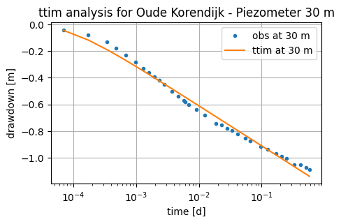
Plotting the model Results

# matplotlib plot for calibration,
plt.semilogx(t1, h1, ".", label="obs at 30 m")  # Plotting the observed drawdown
plt.semilogx(t1, hm1[0], label="ttim at 30 m")  # Simulated drawdown
plt.xlabel("time [d]")
plt.ylabel("drawdown [m]")
plt.title("ttim analysis for Oude Korendijk - Piezometer 30 m")
plt.legend()
plt.grid()

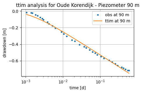
Step 5.2. Calibrate model Parameters with Observation Well 2 (90 m distance)

We proceed to calibrate using only the data from observation well 2. Details on the procedures can be reviewed in step 5.1

ca2 = ttm.Calibrate(ml)
ca2.set_parameter(name="kaq0", initial=10)
ca2.set_parameter(name="Saq0", initial=1e-4)
ca2.series(name="obs2", x=r2, y=0, t=t2, h=h2, layer=0)
ca2.fit()
ca2.parameters

..
...........................
Fit succeeded.

/tmp/ipykernel_1144/974368013.py:2: DeprecationWarning: Setting layers in the parameter name is deprecated. Set the layers= keyword argument for parameter 'kaq0' to silence this warning. The parameter name can still include layer info, but this will be ignored in a future version of TTim.
  ca2.set_parameter(name="kaq0", initial=10)
/tmp/ipykernel_1144/974368013.py:3: DeprecationWarning: Setting layers in the parameter name is deprecated. Set the layers= keyword argument for parameter 'Saq0' to silence this warning. The parameter name can still include layer info, but this will be ignored in a future version of TTim.
  ca2.set_parameter(name="Saq0", initial=1e-4)

	layers	optimal	std	perc_std	pmin	pmax	initial	inhoms	parray
kaq0_0_0	None	71.583273	1.574045	2.198900	-inf	inf	10.0000	None	[[71.58327287853442]]
Saq0_0_0	None	0.000029	0.000002	6.657855	-inf	inf	0.0001	None	[[2.910626378229689e-05]]

print("rmse:", ca2.rmse())
hm2 = ml.head(r2, 0, t2)
plt.semilogx(t2, h2, ".", label="obs at 90 m")
plt.semilogx(t2, hm2[0], label="ttim at 90 m")
plt.xlabel("time [d]")
plt.ylabel("drawdown [m]")
plt.title("ttim analysis for Oude Korendijk - Piezometer 90 m")
plt.legend()
plt.grid()

rmse: 0.022718720854290133

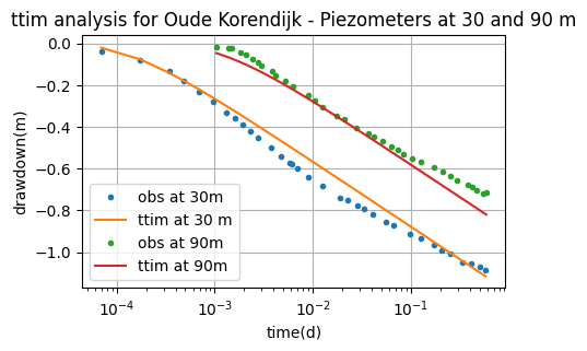
Step 5.3. Calibrate model with two datasets simultaneously

Here we explore the ability of TTim to calibrate the model using more than one observation location.

We achieve this by calling the method .series multiple times to the Calibrate object:

ca = ttm.Calibrate(ml)
ca.set_parameter(name="kaq0", initial=10)
ca.set_parameter(name="Saq0", initial=1e-4)
ca.series(name="obs1", x=r1, y=0, t=t1, h=h1, layer=0)  # Adding well 1
ca.series(name="obs2", x=r2, y=0, t=t2, h=h2, layer=0)  # Adding well 2
ca.fit()
ca.parameters

.....
...
...................
Fit succeeded.

/tmp/ipykernel_1144/210858175.py:2: DeprecationWarning: Setting layers in the parameter name is deprecated. Set the layers= keyword argument for parameter 'kaq0' to silence this warning. The parameter name can still include layer info, but this will be ignored in a future version of TTim.
  ca.set_parameter(name="kaq0", initial=10)
/tmp/ipykernel_1144/210858175.py:3: DeprecationWarning: Setting layers in the parameter name is deprecated. Set the layers= keyword argument for parameter 'Saq0' to silence this warning. The parameter name can still include layer info, but this will be ignored in a future version of TTim.
  ca.set_parameter(name="Saq0", initial=1e-4)

	layers	optimal	std	perc_std	pmin	pmax	initial	inhoms	parray
kaq0_0_0	None	66.088965	1.654963	2.504145	-inf	inf	10.0000	None	[[66.08896475623989]]
Saq0_0_0	None	0.000025	0.000002	9.452155	-inf	inf	0.0001	None	[[2.5409056567587918e-05]]

print("rmse:", ca.rmse())
hs1 = ml.head(r1, 0, t1)
hs2 = ml.head(r2, 0, t2)
plt.semilogx(t1, h1, ".", label="obs at 30m")
plt.semilogx(t1, hs1[0], label="ttim at 30 m")
plt.semilogx(t2, h2, ".", label="obs at 90m")
plt.semilogx(t2, hs2[0], label="ttim at 90m")
plt.xlabel("time(d)")
plt.ylabel("drawdown(m)")
plt.title("ttim analysis for Oude Korendijk - Piezometers at 30 and 90 m")
plt.legend()
plt.grid()

rmse: 0.05005990995553615

Step 6. Calibrate Model with Wellbore Storage

In this continuation, we investigate whether adding wellbore storage improves the fit.

Step 6.1. Reload the model

# unknown parameters: kaq, Saq and rc
ml1 = ttm.ModelMaq(kaq=60, z=[zt, zb], Saq=1e-4, tmin=1e-5, tmax=1)

Step 6.2. Define new Well object with wellbore storage

Now, besides the parameters explained in Step 3, we have to add the radius of the caisson (rc)

w1 = ttm.Well(ml1, xw=0, yw=0, rw=0.2, rc=0.2, tsandQ=[(0, Q)], layers=0)
ml1.solve()

self.neq  1
solution complete

Step 6.3. Calibrate using only the data from observation well 1

The parameters not cited in the .set_paramater method, must be calibrated with the .set_parameter_by_reference method.

Here we use the method .set_parameter_by_reference to calibrate the rc parameter in our well.

.set_parameter_by_reference takes the following arguments:

• name: a string of the parameter name

• parameter: numpy-array with the parameter to be optimized. It should be specified as a reference, for example, in our case: w1.rc[0:] referencing to the parameter rc in object w1.

• initial: float with the initial guess for the parameter value.

• pmin and pmax: floats with the minimum and maximum values allowed. If not specified, these will be defined as -np.inf and np.inf.

ca3 = ttm.Calibrate(ml1)
ca3.set_parameter(name="kaq0", initial=10)
ca3.set_parameter(name="Saq0", initial=1e-4)
ca3.set_parameter_by_reference(
    name="rc", parameter=w1.rc[0:], initial=0.2
)  # , pmin=0.01)
ca3.series(name="obs1", x=r1, y=0, t=t1, h=h1, layer=0)
ca3.fit()
ca3.parameters

.............................
....
...........................
.....
...........................
....
............................
...
............................
...
.............................
..
..............................
..
.............................
..
..............................
..
.............................
Fit succeeded.

/tmp/ipykernel_1144/1266766395.py:2: DeprecationWarning: Setting layers in the parameter name is deprecated. Set the layers= keyword argument for parameter 'kaq0' to silence this warning. The parameter name can still include layer info, but this will be ignored in a future version of TTim.
  ca3.set_parameter(name="kaq0", initial=10)
/tmp/ipykernel_1144/1266766395.py:3: DeprecationWarning: Setting layers in the parameter name is deprecated. Set the layers= keyword argument for parameter 'Saq0' to silence this warning. The parameter name can still include layer info, but this will be ignored in a future version of TTim.
  ca3.set_parameter(name="Saq0", initial=1e-4)

	layers	optimal	std	perc_std	pmin	pmax	initial	inhoms	parray
kaq0_0_0	None	80.945371	1.723759e+00	2.129534	-inf	inf	10.0000	None	[[80.94537078089981]]
Saq0_0_0	None	0.000005	7.903651e-07	14.505488	-inf	inf	0.0001	None	[[5.448731636301055e-06]]
rc	NaN	-0.303964	1.744312e-02	5.738551	-inf	inf	0.2000	NaN	[[-0.3039637890714576]]

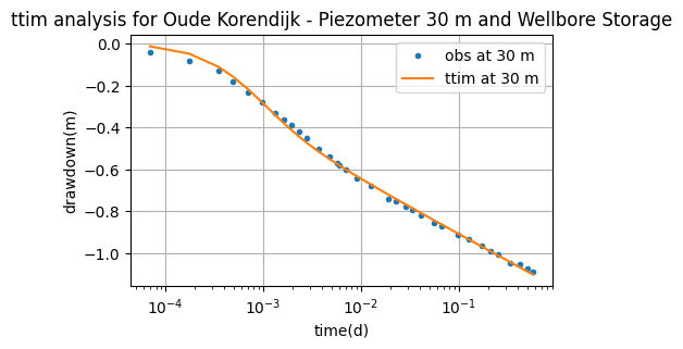
print("rmse:", ca3.rmse())
hm3 = ml1.head(r1, 0, t1)
plt.semilogx(t1, h1, ".", label="obs at 30 m")
plt.semilogx(t1, hm3[0], label="ttim at 30 m")
plt.xlabel("time(d)")
plt.ylabel("drawdown(m)")
plt.title("ttim analysis for Oude Korendijk - Piezometer 30 m and Wellbore Storage")
plt.legend()
plt.grid()

rmse: 0.015273840386221834

ca3.fit_lmfit()

..
.
.............................
.
.
.............................
.
...
...........................
...
..
............................
..
..
............................
..
..
............................
..
..
............................
..
.
.............................
..
.
.............................
...
.
......................
Fit succeeded.

Step 6.4. Calibrate using only the data from observation well 2

Here we repeat the step 6.3 for well 2

ca4 = ttm.Calibrate(ml1)
ca4.set_parameter(name="kaq0", initial=10)
ca4.set_parameter(name="Saq0", initial=1e-4)
ca4.set_parameter_by_reference(name="rc", parameter=w1.rc[0:], initial=0.2, pmin=0.01)
ca4.series(name="obs2", x=r2, y=0, t=t2, h=h2, layer=0)
ca4.fit()
ca4.parameters

.....
.
.
......................
...
....
..
.
......................
..
.....
.
..
.....................
..
.....
..
..
Fit succeeded.

/tmp/ipykernel_1144/1680625426.py:2: DeprecationWarning: Setting layers in the parameter name is deprecated. Set the layers= keyword argument for parameter 'kaq0' to silence this warning. The parameter name can still include layer info, but this will be ignored in a future version of TTim.
  ca4.set_parameter(name="kaq0", initial=10)
/tmp/ipykernel_1144/1680625426.py:3: DeprecationWarning: Setting layers in the parameter name is deprecated. Set the layers= keyword argument for parameter 'Saq0' to silence this warning. The parameter name can still include layer info, but this will be ignored in a future version of TTim.
  ca4.set_parameter(name="Saq0", initial=1e-4)

	layers	optimal	std	perc_std	pmin	pmax	initial	inhoms	parray
kaq0_0_0	None	88.409683	1.462828e+00	1.654601	-inf	inf	10.0000	None	[[88.40968260687684]]
Saq0_0_0	None	0.000011	9.209650e-07	8.164122	-inf	inf	0.0001	None	[[1.1280637263413882e-05]]
rc	NaN	0.677413	2.991638e-02	4.416269	0.01	inf	0.2000	NaN	[[0.6774130763261978]]

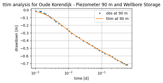
print("rmse:", ca4.rmse())
hm4 = ml1.head(r2, 0, t2)
plt.semilogx(t2, h2, ".", label="obs at 90 m")
plt.semilogx(t2, hm4[0], label="ttim at 90 m")
plt.xlabel("time [d]")
plt.ylabel("drawdown [m]")
plt.title("ttim analysis for Oude Korendijk - Piezometer 90 m and Wellbore Storage")
plt.legend()
plt.grid()

rmse: 0.006219384508921356

Step 6.5. Calibrate model with two datasets simultaneously

Following the same logic from steps 6.3 to 6.4 and the calibration from step 5.3, we can now check the calibration using both wells and wellbore storage.

ca0 = ttm.Calibrate(ml1)
ca0.set_parameter(name="kaq0", initial=10)
ca0.set_parameter(name="Saq0", initial=1e-4)
ca0.set_parameter_by_reference(name="rc", parameter=w1.rc[0:], initial=0.2, pmin=0.01)
ca0.series(name="obs1", x=r1, y=0, t=t1, h=h1, layer=0)
ca0.series(name="obs2", x=r2, y=0, t=t2, h=h2, layer=0)
ca0.fit()
ca0.parameters

.
.
..
..........................
..
...
...........................
.
....
.......
Fit succeeded.

/tmp/ipykernel_1144/3843952862.py:2: DeprecationWarning: Setting layers in the parameter name is deprecated. Set the layers= keyword argument for parameter 'kaq0' to silence this warning. The parameter name can still include layer info, but this will be ignored in a future version of TTim.
  ca0.set_parameter(name="kaq0", initial=10)
/tmp/ipykernel_1144/3843952862.py:3: DeprecationWarning: Setting layers in the parameter name is deprecated. Set the layers= keyword argument for parameter 'Saq0' to silence this warning. The parameter name can still include layer info, but this will be ignored in a future version of TTim.
  ca0.set_parameter(name="Saq0", initial=1e-4)

	layers	optimal	std	perc_std	pmin	pmax	initial	inhoms	parray
kaq0_0_0	None	66.094701	1.668981	2.525135	-inf	inf	10.0000	None	[[66.09470118334973]]
Saq0_0_0	None	0.000025	0.000002	9.571876	-inf	inf	0.0001	None	[[2.539756408228759e-05]]
rc	NaN	0.010016	0.202287	2019.589020	0.01	inf	0.2000	NaN	[[0.010016243921183499]]

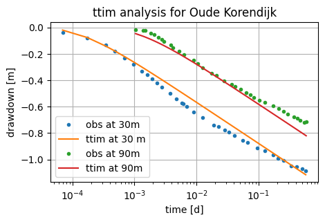
print("rmse:", ca0.rmse())
hs1 = ml1.head(r1, 0, t1)
hs2 = ml1.head(r2, 0, t2)
plt.semilogx(t1, h1, ".", label="obs at 30m")
plt.semilogx(t1, hs1[0], label="ttim at 30 m")
plt.semilogx(t2, h2, ".", label="obs at 90m")
plt.semilogx(t2, hs2[0], label="ttim at 90m")
plt.xlabel("time [d]")
plt.ylabel("drawdown [m]")
plt.title("ttim analysis for Oude Korendijk")
plt.legend()
plt.grid()

rmse: 0.05006500925672784

Step 7. Comparison of Results

Step 7.1. Comparison of model performance and Results with and without wellbore storage

7.1.1. RMSE of the two conceptual models

The following table summarises the RMSE values of the obtained models with and without wellbore storage.

t0 = pd.DataFrame(
    columns=["obs 30 m", "obs 90 m", "obs simultaneously"],
    index=["without rc", "with rc"],
)
t0.loc["without rc", "obs 30 m"] = ca1.rmse()
t0.loc["without rc", "obs 90 m"] = ca2.rmse()
t0.loc["without rc", "obs simultaneously"] = ca.rmse()
t0.loc["with rc", "obs 30 m"] = ca3.rmse()
t0.loc["with rc", "obs 90 m"] = ca4.rmse()
t0.loc["with rc", "obs simultaneously"] = ca0.rmse()

t0.style.set_caption("RMSE of two conceptual models")

RMSE of two conceptual models

	obs 30 m	obs 90 m	obs simultaneously
without rc	0.031660	0.022719	0.050060
with rc	0.015274	0.006219	0.050065

Adding wellbore storage improved the fit performance when used drawdown data of the individual observation wells. However, when calibrated the model with both datasets simultaneously, rc was adjusted to the minimum value. Adding rc did not improve the performance much in this case.

7.1.2. Model comparisons

We can see the summaries of the hydraulic conductivities in the following table.

We will access the parameter values by accessing the .parameters attribute of each Calibrate object.

# Preparing the DataFrame:
t1 = pd.DataFrame(
    columns=["kaq - opt", "kaq - min", "kaq - max", "W. Storage", "Calib. Dataset"]
)
w_storage = [
    "without rc",
    "without rc",
    "without rc",
    "with rc",
    "with rc",
    "with rc",
]
obs_dataset = [
    "obs 30 m",
    "obs 90 m",
    "obs simultaneously",
    "obs 30 m",
    "obs 90 m",
    "obs simultaneously",
]

# Looping through all calibration objects and fetching the desired values
for calib, w_sto, obs_dts in zip(
    [ca1, ca2, ca, ca3, ca4, ca0], w_storage, obs_dataset, strict=False
):
    p = calib.parameters  # Accessing the parameters Dataframe inside the Calibrate object
    tab = pd.DataFrame(
        [
            [
                p.loc["kaq0", "optimal"],
                2 * p.loc["kaq0", "std"],
                2 * p.loc["kaq0", "std"],
                w_sto,
                obs_dts,
            ]
        ],
        columns=["kaq - opt", "kaq - min", "kaq - max", "W. Storage", "Calib. Dataset"],
    )
    t1 = pd.concat(
        (t1 if not t1.empty else None, tab)
    )  # empty rows not allowed in Pandas > 2.1

# Plotting
groups = t1.groupby("W. Storage")
for name, group in groups:
    plt.errorbar(
        x=group["Calib. Dataset"],
        y=group["kaq - opt"],
        yerr=[group["kaq - min"], group["kaq - max"]],
        marker="o",
        linestyle="",
        markersize=12,
        label=name,
    )
plt.legend()
plt.title("Error bar plot of calibrated hydraulic conductivities")
plt.ylabel("K [m/d]")
plt.xlabel("Calibration Dataset")
plt.grid()

---------------------------------------------------------------------------
KeyError                                  Traceback (most recent call last)
File ~/checkouts/readthedocs.org/user_builds/ttim/envs/latest/lib/python3.11/site-packages/pandas/core/indexes/base.py:3641, in Index.get_loc(self, key)
   3640 try:
-> 3641     return self._engine.get_loc(casted_key)
   3642 except KeyError as err:

File pandas/_libs/index.pyx:168, in pandas._libs.index.IndexEngine.get_loc()

File pandas/_libs/index.pyx:197, in pandas._libs.index.IndexEngine.get_loc()

File pandas/_libs/hashtable_class_helper.pxi:7668, in pandas._libs.hashtable.PyObjectHashTable.get_item()

File pandas/_libs/hashtable_class_helper.pxi:7676, in pandas._libs.hashtable.PyObjectHashTable.get_item()

KeyError: 'kaq0'

The above exception was the direct cause of the following exception:

KeyError                                  Traceback (most recent call last)
Cell In[27], line 30
     23 for calib, w_sto, obs_dts in zip(
     24     [ca1, ca2, ca, ca3, ca4, ca0], w_storage, obs_dataset, strict=False
     25 ):
     26     p = calib.parameters  # Accessing the parameters Dataframe inside the Calibrate object
     27     tab = pd.DataFrame(
     28         [
     29             [
---> 30                 p.loc["kaq0", "optimal"],
     31                 2 * p.loc["kaq0", "std"],
     32                 2 * p.loc["kaq0", "std"],
     33                 w_sto,
     34                 obs_dts,
     35             ]
     36         ],
     37         columns=["kaq - opt", "kaq - min", "kaq - max", "W. Storage", "Calib. Dataset"],
     38     )
     39     t1 = pd.concat(
     40         (t1 if not t1.empty else None, tab)
     41     )  # empty rows not allowed in Pandas > 2.1
     43 # Plotting

File ~/checkouts/readthedocs.org/user_builds/ttim/envs/latest/lib/python3.11/site-packages/pandas/core/indexing.py:1199, in _LocationIndexer.__getitem__(self, key)
   1197     key = tuple(com.apply_if_callable(x, self.obj) for x in key)
   1198     if self._is_scalar_access(key):
-> 1199         return self.obj._get_value(*key, takeable=self._takeable)
   1200     return self._getitem_tuple(key)
   1201 else:
   1202     # we by definition only have the 0th axis

File ~/checkouts/readthedocs.org/user_builds/ttim/envs/latest/lib/python3.11/site-packages/pandas/core/frame.py:4495, in DataFrame._get_value(self, index, col, takeable)
   4489 series = self._get_item(col)
   4491 if not isinstance(self.index, MultiIndex):
   4492     # CategoricalIndex: Trying to use the engine fastpath may give incorrect
   4493     #  results if our categories are integers that dont match our codes
   4494     # IntervalIndex: IntervalTree has no get_loc
-> 4495     row = self.index.get_loc(index)
   4496     return series._values[row]
   4498 # For MultiIndex going through engine effectively restricts us to
   4499 #  same-length tuples; see test_get_set_value_no_partial_indexing

File ~/checkouts/readthedocs.org/user_builds/ttim/envs/latest/lib/python3.11/site-packages/pandas/core/indexes/base.py:3648, in Index.get_loc(self, key)
   3643     if isinstance(casted_key, slice) or (
   3644         isinstance(casted_key, abc.Iterable)
   3645         and any(isinstance(x, slice) for x in casted_key)
   3646     ):
   3647         raise InvalidIndexError(key) from err
-> 3648     raise KeyError(key) from err
   3649 except TypeError:
   3650     # If we have a listlike key, _check_indexing_error will raise
   3651     #  InvalidIndexError. Otherwise we fall through and re-raise
   3652     #  the TypeError.
   3653     self._check_indexing_error(key)

KeyError: 'kaq0'

The Errorbar plot shows that the Hydraulic Conductivities calculated are significantly higher with wellbore storage than without when considering the individual wells datasets for calibration.

As for the dataset using both obs wells at the same time, the calibration results have no significant differences.

Both scenarios with and without wellbore storage showed lower values for the calibrated model using both observations, calibration with a single well are overestimated.

Step 7.2. Compare TTim to results of K&dR, AQTEOLV and MLU:

The final important step is to compare the data obtained from this model with the data from other Aquifer Analysis software. Yang (2020) compared TTim results with the published results in Kruseman and de Ridder (1990), here abbreviated to K&dR, and with the results obtained from the software AQTESOLV (Duffield, 2007) and MLU (Carlson & Randall, 2012).

t = pd.DataFrame(
    columns=["k [m/d]", "Ss [1/m]", "RMSE"], index=["K&dR", "TTim", "AQTESOLV", "MLU"]
)
t.loc["TTim"] = np.append(ca.parameters["optimal"].values, ca.rmse())
t.loc["AQTESOLV"] = [66.086, 2.541e-05, 0.05006]
t.loc["MLU"] = [66.850, 2.400e-05, 0.05083]
t.loc["K&dR"] = [55.71429, 1.7e-4, "-"]
t.style.set_caption("Comparison of Model Results with different Softwares")

Comparison of Model Results with different Softwares

	k [m/d]	Ss [1/m]	RMSE
K&dR	55.714290	0.000170	-
TTim	66.088965	0.000025	0.050060
AQTESOLV	66.086000	0.000025	0.050060
MLU	66.850000	0.000024	0.050830

Results show good agreement between different analysis programs, including TTim. The values from Kruseman and de Ridder (1990) were obtained through Thiem’s approximation. They seem to be an underestimation, as the pumping never reached steady-state conditions.

References

• Bakker, M. Semi-analytic modeling of transient multi-layer flow with TTim. Hydrogeol J 21, 935–943 (2013). https://doi.org/10.1007/s10040-013-0975-2

• Carlson F, Randall J (2012) MLU: a Windows application for the analysis of aquifer tests and the design of well fields in layered systems. Ground Water 50(4):504–510

• Duffield, G.M., 2007. AQTESOLV for Windows Version 4.5 User’s Guide, HydroSOLVE, Inc., Reston, VA.

• Newville, M.,Stensitzki, T., Allen, D.B., Ingargiola, A. (2014) LMFIT: Non Linear Least-Squares Minimization and Curve Fitting for Python.https://dx.doi.org/10.5281/zenodo.11813. https://lmfit.github.io/lmfit-py/intro.html (last access: August,2021).

• Kruseman, G.P., De Ridder, N.A., Verweij, J.M., 1970. Analysis and evaluationof pumping test data. volume 11. International institute for land reclamation and improvement The Netherlands.

• Yang, Xinzhu (2020) Application and comparison of different methodsfor aquifer test analysis using TTim. Master Thesis, Delft University of Technology (TUDelft), Delft, The Netherlands.