Well near a straight river

import matplotlib.pyplot as plt
import numpy as np

import ttim

plt.rcParams["font.size"] = 8.0

Consider a well in the middle aquifer of a three aquifer system located at \((x,y)=(0,0)\). The well starts pumping at time \(t=0\) at a discharge of \(Q=1000\) m\(^3\)/d. Aquifer properties are the shown in table 3 (same as exercise 2). A stream runs North-South along the line \(x=50\). The head along the stream is fixed.

Table 3 - Aquifer properties for exercise 3.

Layer	\(k\) (m/d)	\(c\) (d)	\(S\)	\(S_s\)	\(z_t\) (m)	\(z_b\) (m)
Aquifer 0	1		0.1		25	20
Leaky layer 1		1000		0	20	18
Aquifer 1	20			0.0001	18	10
Leaky layer 2		2000		0	10	8
Aquifer 2	2			0.0001	8	0

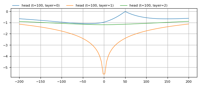
Exercise 3a

Model a 1000 m long section of the stream using 12 linesinks with \(y\)-endpoints at [-500,-300,-200,-100,-50,0,50,100,200,300,500]. Create a cross-section of the head along \(y=0\) from \(x=-200\) to \(x=200\) in all 3 layers.

ml = ttim.ModelMaq(
    kaq=[1, 20, 2],
    z=[25, 20, 18, 10, 8, 0],
    c=[1000, 2000],
    Saq=[0.1, 1e-4, 1e-4],
    Sll=[0, 0],
    phreatictop=True,
    tmin=0.1,
    tmax=1000,
)
w = ttim.Well(ml, xw=0, yw=0, rw=0.2, tsandQ=[(0, 1000)], layers=1, label="well 1")
yls = [-500, -300, -200, -100, -50, 0, 50, 100, 200, 300, 500]
xls = 50 * np.ones(len(yls))
ls1 = ttim.HeadLineSinkString(
    ml, list(zip(xls, yls, strict=False)), tsandh="fixed", layers=0, label="river"
)
ml.solve()
ml.plots.head_along_line(
    x1=-200, x2=200, npoints=100, t=100, layers=[0, 1, 2], sstart=-200, figsize=(8, 3)
);

self.neq  11
solution complete

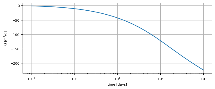
Exercise 3b

Compute the discharge of the stream section (the stream depletion) as a function of time from \(t=0.1\) till \(t=1000\) days.

t = np.logspace(-1, 3, 100)
Q = ls1.discharge(t)
plt.figure(figsize=(8, 3))
plt.semilogx(t, Q[0])
plt.ylabel("Q [m$^3$/d]")
plt.xlabel("time [days]")
plt.grid()

# # check if dischargeold function produces same result
# # can be removed after version 0.6.6
# t = np.logspace(-1, 3, 100)
# Q = ls1.dischargeold(t)
# plt.semilogx(t, Q[0])
# plt.ylabel('Q [m$^3$/d]')
# plt.xlabel('time [days]');

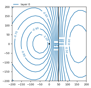
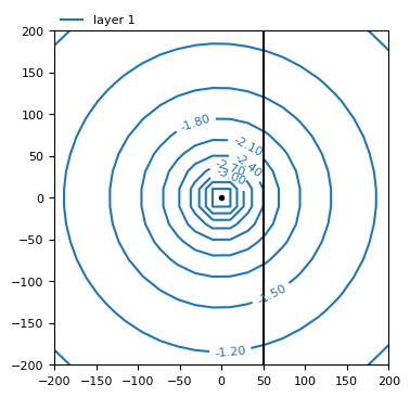
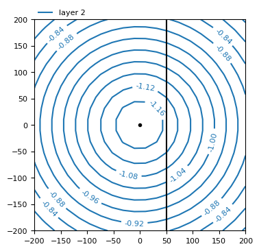
Exercise 3c

Make a contour plot of each layer after 100 days of pumping. Use 20 grid points in each direction (this may take a little time).

for ilay in [0, 1, 2]:
    ml.plots.contour(
        win=[-200, 200, -200, 200],
        ngr=[20, 20],
        t=100,
        layers=ilay,
        levels=10,
        color="C0",
        labels=True,
        decimals=2,
        figsize=(4, 4),
    )

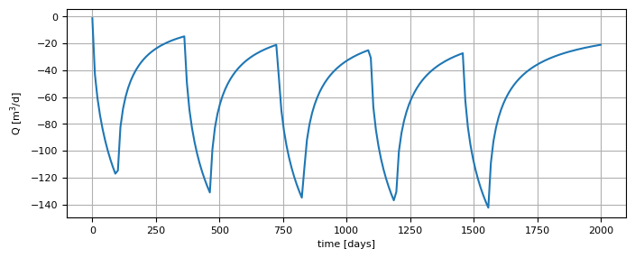
Exercise 3d

The discharge of the well is \(Q=1000\) m\(^3\)/d for 100 days every summer. Compute the stream depletion for a five year period.

ml = ttim.ModelMaq(
    kaq=[1, 20, 2],
    z=[25, 20, 18, 10, 8, 0],
    c=[1000, 2000],
    Saq=[0.1, 1e-4, 1e-4],
    Sll=[0, 0],
    phreatictop=True,
    tmin=0.1,
    tmax=2000,
)
tsandQ = [
    (0, 1000),
    (100, 0),
    (365, 1000),
    (465, 0),
    (730, 1000),
    (830, 0),
    (1095, 1000),
    (1195, 0),
    (1460, 1000),
    (1560, 0),
]
w = ttim.Well(ml, xw=0, yw=0, rw=0.2, tsandQ=tsandQ, layers=1, label="well 1")
yls = [-500, -300, -200, -100, -50, 0, 50, 100, 200, 300, 500]
xls = 50 * np.ones(len(yls))
ls1 = ttim.HeadLineSinkString(
    ml, list(zip(xls, yls, strict=False)), tsandh="fixed", layers=0, label="river"
)
ml.solve()

t = np.linspace(0.1, 2000, 200)
Q = ls1.discharge(t)
plt.figure(figsize=(8, 3))
plt.plot(t, Q[0])
plt.ylabel("Q [m$^3$/d]")
plt.xlabel("time [days]")
plt.grid()

self.neq  11
solution complete