2. Confined Aquifer Test - Grindley#

This test is taken from AQTESOLV examples.

Introduction and Conceptual Model#

In this example, we reproduce the work of Yang (2020) to use the pumping test data to demonstrate how TTim can be used to model and analyze pumping tests in a single layer, confined setting. Furthermore, we compare the performance of TTim with other transient well hydraulics software AQTESOLV (Duffield, 2007) and MLU (Carlson and Randall, 2012).

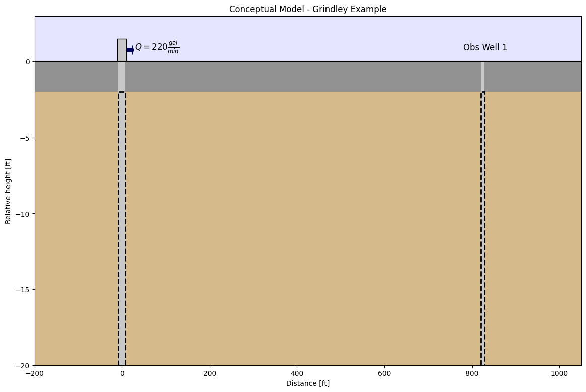
This example is a pumping test conducted in 1953 in Grindley, Illinois, US. It was reported by Walton (1962). The aquifer is an 18 ft thickness sand and gravel layer under confined conditions. The pumping well fully penetrates the formation, and pumping was conducted for 8 hours at a rate of 220 gallons per minute. The effect of pumping was observed at observation well 1, located 824 ft away from the well.

The time-drawdown data for the observation well was obtained from AQTESOLV documentation (Duffield, 2007), while data from the pumping well was obtained from the original paper from Walton (1962). Following AQTESOLV documentation (Duffield, 2007), we have assumed that both well and observation well radii are 0.5 ft.

A simplified cross-section of the model area can be seen below:

Show code cell source

Hide code cell source

import matplotlib.pyplot as plt
import numpy as np

##Now printing the conceptual model figure:

fig = plt.figure(figsize=(14, 9))
ax = fig.add_subplot(1, 1, 1)
# sky
sky = plt.Rectangle((-200, 0), width=1400, height=3, fc="b", zorder=0, alpha=0.1)
ax.add_patch(sky)

# Aquifer:
ground = plt.Rectangle(
    (-200, -20),
    width=1400,
    height=18,
    fc=np.array([209, 179, 127]) / 255,
    zorder=0,
    alpha=0.9,
)
ax.add_patch(ground)

# Confining bed:
confining_unit = plt.Rectangle(
    (-200, -2),
    width=1400,
    height=2,
    fc=np.array([100, 100, 100]) / 255,
    zorder=0,
    alpha=0.7,
)
ax.add_patch(confining_unit)
well = plt.Rectangle(
    (-8, -20), width=16, height=20, fc=np.array([200, 200, 200]) / 255, zorder=1
)
ax.add_patch(well)

# Wellhead
wellhead = plt.Rectangle(
    (-10, 0), width=20, height=1.5, fc=np.array([200, 200, 200]) / 255, zorder=2, ec="k"
)
ax.add_patch(wellhead)

# Screen for the well:
screen = plt.Rectangle(
    (-8, -20),
    width=16,
    height=18,
    fc=np.array([200, 200, 200]) / 255,
    alpha=1,
    zorder=2,
    ec="k",
    ls="--",
)
screen.set_linewidth(2)
ax.add_patch(screen)
pumping_arrow = plt.Arrow(x=10, y=0.75, dx=16, dy=0, color="#00035b")
ax.add_patch(pumping_arrow)
ax.text(x=29, y=0.75, s=r"$ Q = 220 \frac{gal}{min}$", fontsize="large")
# Piezometers
piez1 = plt.Rectangle(
    (820, -20), width=8, height=20, fc=np.array([200, 200, 200]) / 255, zorder=1
)
screen_piez_1 = plt.Rectangle(
    (820, -20),
    width=8,
    height=18,
    fc=np.array([200, 200, 200]) / 255,
    alpha=1,
    zorder=2,
    ec="k",
    ls="--",
)
screen_piez_1.set_linewidth(2)

ax.add_patch(piez1)

ax.add_patch(screen_piez_1)

# last line
line = plt.Line2D(xdata=[-200, 1200], ydata=[0, 0], color="k")
ax.add_line(line)
ax.text(x=780, y=0.75, s="Obs Well 1", fontsize="large")

ax.set_xlim([-200, 1050])
ax.set_ylim([-20, 3])
ax.set_xlabel("Distance [ft]")
ax.set_ylabel("Relative height [ft]")
ax.set_title("Conceptual Model - Grindley Example");

../_images/a8d26c719d427c50d9e7b9b9177988d89c15561e17d0961fda2398435f8c5fe9.png

Step 1. Load required libraries#

import matplotlib.pyplot as plt
import numpy as np
import pandas as pd

import ttim

Step 2. Set basic parameters#

We will work with time in days and length in meters from this step onwards
The parameters below have already been converted to m and days.

b = -5.4846  # aquifer thickness in m (Converted from 18 ft)
Q = 1199.218  # constant discharge in m^3/d (Converted from 220 gallons/minute)
r = 251.1552  # distance from observation well to test well in m (converted from 824 ft)
rw = 0.1524  # screen radius of test well in m (Converted from 0.5 ft)

Step 3. Load data of observation and pumping well#

The preferred method of loading data into TTim is to use numpy arrays.

The data is in a text file where the first column is the time data in days and the second column is the drawdown in meters

The observation well is referred to as Well 1 and the pumping well as Well 3.

For each piezometer, we will load the data as a numpy array and split time and drawdown into two different 1d arrays.

# Loading Observation well (Well 1)
data1 = np.loadtxt("data/gridley_well_1.txt")
t1 = data1[:, 0]
h1 = data1[:, 1]

# Loading Pumping Well data (Well 3)
data2 = np.loadtxt("data/gridley_well_3.txt")
t2 = data2[:, 0]
h2 = data2[:, 1]

Step 4. Creating a TTim conceptual model#

In this example, we are using the ModelMaq model to conceptualize our aquifer. ModelMaq defines the aquifer system as a stacked vertical sequence of aquifers and leaky layers (aquifer-leaky layer, aquifer-leaky layer etc). A thorough explanation of the ModelMaq and TTim one-layer modelling conceptualization is given in the notebook: Confined 1 - Oude Korendijk

ml = ttim.ModelMaq(kaq=10, z=[0, b], Saq=0.001, tmin=0.001, tmax=1, topboundary="conf")
w = ttim.Well(ml, xw=0, yw=0, rw=rw, tsandQ=[(0, Q)], layers=0)
ml.solve()

self.neq  1
solution complete

Step 5. Calibration#

The calibration workflow has been described in detail in the notebook: Confined 1 - Oude Korendijk

Step 5.1. Calibration Using the Observation Well#

We begin the calibration using the data from observation well (well 1) as our data set.

# unknown parameters: kaq, Saq
ca_0 = ttim.Calibrate(ml)  # Create the Calibrate object, calling the model to the object
ca_0.set_parameter(name="kaq0", initial=10)  # Setting the parameters for calibration
ca_0.set_parameter(name="Saq0", initial=1e-4)
ca_0.series(name="obs1", x=r, y=0, t=t1, h=h1, layer=0)  # Setting the observation data
ca_0.fit(
    report=True
)  # Fitting the model. We can hide the message below setting report = False

...............................
Fit succeeded.
[[Fit Statistics]]
    # fitting method   = leastsq
    # function evals   = 28
    # data points      = 22
    # variables        = 2
    chi-square         = 0.01702154
    reduced chi-square = 8.5108e-04
    Akaike info crit   = -153.615001
    Bayesian info crit = -151.432916
[[Variables]]
    kaq0_0_0:  22.4340744 +/- 0.22268739 (0.99%) (init = 10)
    Saq0_0_0:  3.8208e-06 +/- 7.4239e-08 (1.94%) (init = 0.0001)
[[Correlations]] (unreported correlations are < 0.100)
    C(kaq0_0_0, Saq0_0_0) = -0.8829

/tmp/ipykernel_1146/2829729724.py:3: DeprecationWarning: Setting layers in the parameter name is deprecated. Set the layers= keyword argument for parameter 'kaq0' to silence this warning. The parameter name can still include layer info, but this will be ignored in a future version of TTim.
  ca_0.set_parameter(name="kaq0", initial=10)  # Setting the parameters for calibration
/tmp/ipykernel_1146/2829729724.py:4: DeprecationWarning: Setting layers in the parameter name is deprecated. Set the layers= keyword argument for parameter 'Saq0' to silence this warning. The parameter name can still include layer info, but this will be ignored in a future version of TTim.
  ca_0.set_parameter(name="Saq0", initial=1e-4)

The results from calibration are stored in the .parameters attribute of the calibration object. We can also call the .rmse method to check the fitting error (RMSE)

display(ca_0.parameters)
print("rmse:", ca_0.rmse())

	layers	optimal	std	perc_std	pmin	pmax	initial	inhoms	parray
kaq0_0_0	None	22.434074	2.226874e-01	0.992630	-inf	inf	10.0000	None	[[22.434074359199766]]
Saq0_0_0	None	0.000004	7.423858e-08	1.943034	-inf	inf	0.0001	None	[[3.820756380848479e-06]]

rmse: 0.02781557661480393

Now, we plot the model with our observation data:

First, we have to compute the model calculated heads at the observation location. For this, we use the .headmethod in the model object (ml). This method takes the following arguments
- the positions x and y of the piezometric well (or any other point of interest). In our case, our well is located at position x= r1 and y = 0.
- the time intervals, defined by the numpy array t, for the computation of the heads. In our case, this is defined by the variable t1.
- Another optional input is layers, which can be a list, integer or an array defining the model layers. When we do not assign anything, the head is computed for all layers.

The output is a numpy array with dimensions (nl,nt), where nl is the number of layers and nt is the number of time intervals.

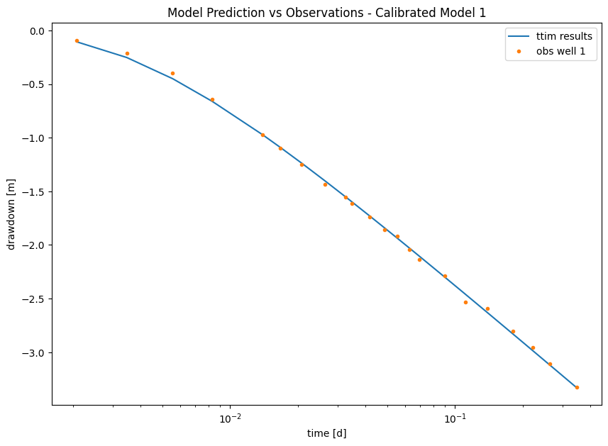
Now, we can compare both observations and predictions in a plot:

hm_0 = ml.head(x=r, y=0, t=t1)  # Compute heads at observation well location
plt.figure(figsize=(10, 7))
plt.semilogx(t1, hm_0[0], label="ttim results")  # Plotting TTim model Results
plt.semilogx(t1, h1, ".", label="obs well 1")  # Plotting Observed points
plt.xlabel("time [d]")
plt.ylabel("drawdown [m]")
plt.title("Model Prediction vs Observations - Calibrated Model 1")
plt.legend();

../_images/72239b4308a22291d55b33bc3f54fe626c1f18e3474e623081026ac5149c5000.png

Now let’s check how it performs with the Pumping Well data:

hm_0_2 = ml.head(x=0, y=0, t=t2)  # Compute heads at observation well location
plt.figure(figsize=(8, 5))
plt.semilogx(t2, hm_0_2[0], label="ttim results")  # Plotting TTim model Results
plt.semilogx(t2, h2, ".", label="well 3")  # Plotting Observed points
plt.xlabel("time [d]")
plt.ylabel("drawdown [m]")
plt.title(
    "Model Prediction vs Observations - Calibrated Model 1, Results in the Pumping Well"
)
plt.legend();

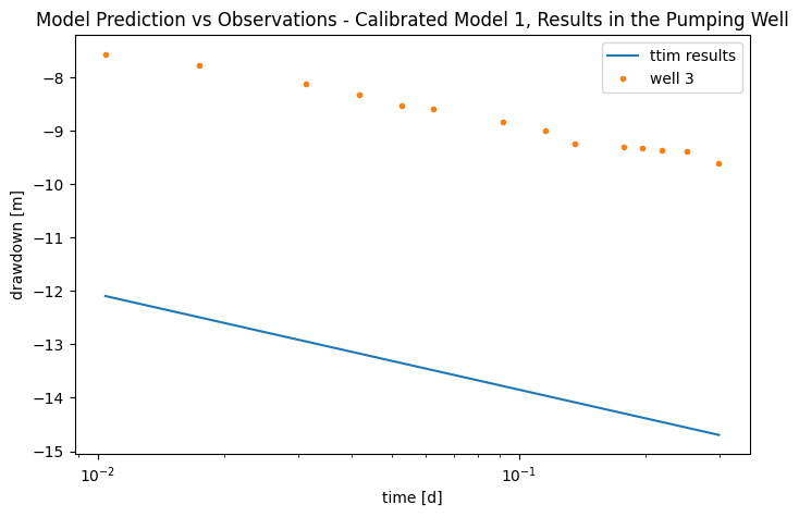
../_images/b48d34f94b17b671833dde4ad583f592327e8cfb16c920f8ab1f58f22dcf904a.png

As we can see, although the model presented an initial good fit, when we challenged it with an outside sample, it performed poorly.

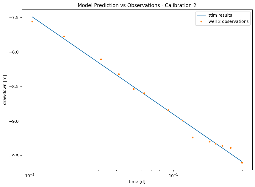
Step 5.2. Calibration using the Pumping Well data#

We proceed to calibrate using only the data from the pumping well (Well 3). The initial inputs can be checked in step 5.1

# unknown parameters: kaq, Saq
ca_1 = ttim.Calibrate(ml)
ca_1.set_parameter(name="kaq0", initial=10)
ca_1.set_parameter(name="Saq0", initial=1e-4)
ca_1.series(name="well3", x=0, y=0, t=t2, h=h2, layer=0)
ca_1.fit(report=True)

...................................
Fit succeeded.
[[Fit Statistics]]
    # fitting method   = leastsq
    # function evals   = 32
    # data points      = 14
    # variables        = 2
    chi-square         = 0.04383766
    reduced chi-square = 0.00365314
    Akaike info crit   = -76.7284713
    Bayesian info crit = -75.4503567
[[Variables]]
    kaq0_0_0:  27.8997730 +/- 0.73085951 (2.62%) (init = 10)
    Saq0_0_0:  1.7014e-04 +/- 5.8194e-05 (34.20%) (init = 0.0001)
[[Correlations]] (unreported correlations are < 0.100)
    C(kaq0_0_0, Saq0_0_0) = -0.9971

/tmp/ipykernel_1146/1587861927.py:3: DeprecationWarning: Setting layers in the parameter name is deprecated. Set the layers= keyword argument for parameter 'kaq0' to silence this warning. The parameter name can still include layer info, but this will be ignored in a future version of TTim.
  ca_1.set_parameter(name="kaq0", initial=10)
/tmp/ipykernel_1146/1587861927.py:4: DeprecationWarning: Setting layers in the parameter name is deprecated. Set the layers= keyword argument for parameter 'Saq0' to silence this warning. The parameter name can still include layer info, but this will be ignored in a future version of TTim.
  ca_1.set_parameter(name="Saq0", initial=1e-4)

# ca_1.parameters
print("rmse:", ca_1.rmse())

rmse: 0.05595767430212018

hm_1 = ml.head(0, 0, t2)
plt.figure(figsize=(10, 7))
plt.semilogx(t2, hm_1[0], label="ttim results")
plt.semilogx(t2, h2, ".", label="well 3 observations")
plt.xlabel("time [d]")
plt.ylabel("drawdown [m]")
plt.title("Model Prediction vs Observations - Calibration 2")
plt.legend();

../_images/bf1a55b0064d166d9199be350f7b79f71bb5752cf6492befdfbdc0446bb61b14.png

Step 5.3. Model Calibration with both datasets#

We now will proceed to calibrate the model using both datasets at the same time. We begin by creating a new model so we can compare the different results later:

ml_1 = ttim.ModelMaq(kaq=10, z=[0, b], Saq=0.001, tmin=0.001, tmax=1, topboundary="conf")
w_1 = ttim.Well(ml_1, xw=0, yw=0, rw=rw, tsandQ=[(0, Q)], layers=0)
ml_1.solve()

self.neq  1
solution complete

We now create a new Calibrate object. The difference from the previous calibration objects is that now we add a second observation series to the object:

ca_2 = ttim.Calibrate(ml_1)
ca_2.set_parameter(name="kaq0", initial=10)
ca_2.set_parameter(name="Saq0", initial=1e-4, pmin=0)
ca_2.series(name="obs1", x=r, y=0, t=t1, h=h1, layer=0)  # Adding observation Well 1
ca_2.series(name="well3", x=0, y=0, t=t2, h=h2, layer=0)  # Adding Pumping Well (Well 3)
ca_2.fit(report=True)

.................................
Fit succeeded.
[[Fit Statistics]]
    # fitting method   = leastsq
    # function evals   = 30
    # data points      = 36
    # variables        = 2
    chi-square         = 2.65994253
    reduced chi-square = 0.07823360
    Akaike info crit   = -89.7877191
    Bayesian info crit = -86.6206813
[[Variables]]
    kaq0_0_0:  38.0492402 +/- 0.52460206 (1.38%) (init = 10)
    Saq0_0_0:  1.2468e-06 +/- 2.0176e-07 (16.18%) (init = 0.0001)
[[Correlations]] (unreported correlations are < 0.100)
    C(kaq0_0_0, Saq0_0_0) = -0.7693

/tmp/ipykernel_1146/1681425234.py:2: DeprecationWarning: Setting layers in the parameter name is deprecated. Set the layers= keyword argument for parameter 'kaq0' to silence this warning. The parameter name can still include layer info, but this will be ignored in a future version of TTim.
  ca_2.set_parameter(name="kaq0", initial=10)
/tmp/ipykernel_1146/1681425234.py:3: DeprecationWarning: Setting layers in the parameter name is deprecated. Set the layers= keyword argument for parameter 'Saq0' to silence this warning. The parameter name can still include layer info, but this will be ignored in a future version of TTim.
  ca_2.set_parameter(name="Saq0", initial=1e-4, pmin=0)

display(ca_2.parameters)
print("rmse:", ca_2.rmse())

	layers	optimal	std	perc_std	pmin	pmax	initial	inhoms	parray
kaq0_0_0	None	38.049240	5.246021e-01	1.378745	-inf	inf	10.0000	None	[[38.04924016631566]]
Saq0_0_0	None	0.000001	2.017604e-07	16.182093	0.0	inf	0.0001	None	[[1.2468126702191995e-06]]

rmse: 0.2718221707825475

The parameters are quite different from the first two models. We can also see that the errors have increased significantly. Let’s plot the model results with the observations and check why we have large errors:

hm1_2 = ml.head(r, 0, t1)
hm2_2 = ml.head(0, 0, t2)
plt.figure(figsize=(10, 7))
plt.semilogx(t1, hm1_2[0], label="ttim model results - obs 1")
plt.semilogx(t1, h1, ".", label="obs1")
plt.semilogx(t2, hm2_2[0], label="ttim model results - well 3")
plt.semilogx(t2, h2, ".", label="well3")
plt.xlabel("time [d]")
plt.ylabel("drawdown [m]")
plt.title("Model Prediction vs Observations - Calibration 3")
plt.legend();

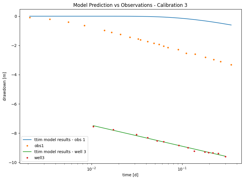
../_images/1baf3813fb1e723938f3f01eab810dc2afdc8c2aa75b3b22fdb396c04095c066.png

As seen in the Figure above, TTim could not adjust both curves simultaneously and ended up fitting only Well 3.

Fortunately, in TTim, we can improve this fit by simulating skin resistance and wellbore storage.

Step 5.4. Model Calibration with skin resistance and wellbore storage#

For this, we create a new model and add two extra parameters to the Well object:

The radius of the caisson rc, which we use to simulate wellbore storage. In this case, we use a value in meters (float). The function of the radius of the caisson to account for wellbore storage is explained in the previous notebook: Confined 1 - Oude Korendijk;
The skin resistance res, a float value unit of time (in our case days). The effect of the skin resistance is explained in Confined 1 - Oude Korendijk.

ml_2 = ttim.ModelMaq(kaq=10, z=[0, b], Saq=0.001, tmin=0.001, tmax=1, topboundary="conf")
w_2 = ttim.Well(ml_2, xw=0, yw=0, rw=rw, rc=0.2, res=0.2, tsandQ=[(0, Q)], layers=0)
ml_2.solve()

self.neq  1
solution complete

Here we use the method .set_parameter_by_reference to calibrate the rc and res parameters in our well.

.set_parameter_by_reference takes the following arguments:

name: a string of the parameter name
parameter: numpy-array with the parameter to be optimized. It should be specified as a reference, for example, in our case: w1.rc[0:] referencing to the parameter rc in object w1.
initial: float with the initial guess for the parameter value.
pmin and pmax: floats with the minimum and maximum values allowed. If not specified, these will be -np.inf and np.inf.

ca_3 = ttim.Calibrate(ml_2)
ca_3.set_parameter(name="kaq0", initial=10)
ca_3.set_parameter(name="Saq0", initial=1e-4, pmin=0)
ca_3.set_parameter_by_reference(
    name="res", parameter=w_2.res, initial=0.2, pmin=0
)  # Here we add pmin = 0 to avoid unrealistic values
ca_3.set_parameter_by_reference(name="rc", parameter=w_2.rc, initial=0.2)
ca_3.series(name="obs1", x=r, y=0, t=t1, h=h1, layer=0)
ca_3.series(name="obs3", x=0, y=0, t=t2, h=h2, layer=0)
ca_3.fit(report=True)

...
..
.......................................
.....
...
.........................................
......
.
..........................................
.....
..
.......................
Fit succeeded.
[[Fit Statistics]]
    # fitting method   = leastsq
    # function evals   = 169
    # data points      = 36
    # variables        = 4
    chi-square         = 1.29522403
    reduced chi-square = 0.04047575
    Akaike info crit   = -111.694069
    Bayesian info crit = -105.359994
[[Variables]]
    kaq0_0_0:  38.2996120 +/- 0.39757184 (1.04%) (init = 10)
    Saq0_0_0:  8.9401e-07 +/- 1.1941e-07 (13.36%) (init = 0.0001)
    res:       5.0025e-07 +/- 0.00124718 (249311.68%) (init = 0.2)
    rc:        0.42223234 +/- 0.04545438 (10.77%) (init = 0.2)
[[Correlations]] (unreported correlations are < 0.100)
    C(res, rc)            = -0.7841
    C(kaq0_0_0, Saq0_0_0) = -0.7392
    C(Saq0_0_0, rc)       = -0.3203
    C(Saq0_0_0, res)      = +0.2017

/tmp/ipykernel_1146/178239275.py:2: DeprecationWarning: Setting layers in the parameter name is deprecated. Set the layers= keyword argument for parameter 'kaq0' to silence this warning. The parameter name can still include layer info, but this will be ignored in a future version of TTim.
  ca_3.set_parameter(name="kaq0", initial=10)
/tmp/ipykernel_1146/178239275.py:3: DeprecationWarning: Setting layers in the parameter name is deprecated. Set the layers= keyword argument for parameter 'Saq0' to silence this warning. The parameter name can still include layer info, but this will be ignored in a future version of TTim.
  ca_3.set_parameter(name="Saq0", initial=1e-4, pmin=0)

display(ca_3.parameters)
print("rmse:", ca_3.rmse())

	layers	optimal	std	perc_std	pmin	pmax	initial	inhoms	parray
kaq0_0_0	None	3.829961e+01	3.975718e-01	1.038057	-inf	inf	10.0000	None	[[38.29961203674786]]
Saq0_0_0	None	8.940113e-07	1.194081e-07	13.356441	0.0	inf	0.0001	None	[[8.94011342511547e-07]]
res	NaN	5.002501e-07	1.247182e-03	249311.684612	0.0	inf	0.2000	NaN	[[5.002500662598663e-07]]
rc	NaN	4.222323e-01	4.545438e-02	10.765254	-inf	inf	0.2000	NaN	[[0.4222323399293044]]

rmse: 0.18967984965611256

hm1_3 = ml_2.head(r, 0, t1)
hm2_3 = ml_2.head(0, 0, t2)
plt.figure(figsize=(10, 7))
plt.semilogx(t1, hm1_3[0], label="ttim model results - obs 1")
plt.semilogx(t1, h1, ".", label="obs1")
plt.semilogx(t2, hm2_3[0], label="ttim model results - well 3")
plt.semilogx(t2, h2, ".", label="well3")
plt.xlabel("time [d]")
plt.ylabel("drawdown [m]")
plt.title("Model Prediction vs Observations - Calibration 4")
plt.legend();

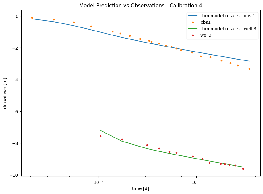
../_images/d1cd50e049ad9a19ce39361efae300ed5a0a8cde9a52db56c67f32c6338d2d40.png

Here, we see in the picture that we have significantly improved both models by adding the resistance and the wellbore storage. We can make a critique of our current model that the adjusted resistance value is too low and with a very high standard deviation (adjusted parameters). Let’s now disregard the skin resistance and check our model performance.

Step 5.5. Model Calibration with wellbore storage#

We start by creating a model and adding a well with no resistance:

ml_3 = ttim.ModelMaq(kaq=10, z=[0, b], Saq=0.001, tmin=0.001, tmax=1, topboundary="conf")
w_3 = ttim.Well(ml_3, xw=0, yw=0, rw=rw, rc=0.2, res=0, tsandQ=[(0, Q)], layers=0)
ml_3.solve()

self.neq  1
solution complete

Now we calibrate without changing the resistance parameter

ca_4 = ttim.Calibrate(ml_3)
ca_4.set_parameter(name="kaq0", initial=10)
ca_4.set_parameter(name="Saq0", initial=1e-4, pmin=0)
ca_4.set_parameter_by_reference(name="rc", parameter=w_3.rc, initial=0.2)
ca_4.series(name="obs1", x=r, y=0, t=t1, h=h1, layer=0)
ca_4.series(name="obs3", x=0, y=0, t=t2, h=h2, layer=0)
ca_4.fit(report=True)

..
....
.................................
Fit succeeded.
[[Fit Statistics]]
    # fitting method   = leastsq
    # function evals   = 36
    # data points      = 36
    # variables        = 3
    chi-square         = 1.29522639
    reduced chi-square = 0.03924928
    Akaike info crit   = -113.694004
    Bayesian info crit = -108.943447
[[Variables]]
    kaq0_0_0:  38.2996071 +/- 0.39115777 (1.02%) (init = 10)
    Saq0_0_0:  8.9399e-07 +/- 1.1517e-07 (12.88%) (init = 0.0001)
    rc:        0.42216850 +/- 0.02778786 (6.58%) (init = 0.2)
[[Correlations]] (unreported correlations are < 0.100)
    C(kaq0_0_0, Saq0_0_0) = -0.7468
    C(Saq0_0_0, rc)       = -0.2669

/tmp/ipykernel_1146/160360364.py:2: DeprecationWarning: Setting layers in the parameter name is deprecated. Set the layers= keyword argument for parameter 'kaq0' to silence this warning. The parameter name can still include layer info, but this will be ignored in a future version of TTim.
  ca_4.set_parameter(name="kaq0", initial=10)
/tmp/ipykernel_1146/160360364.py:3: DeprecationWarning: Setting layers in the parameter name is deprecated. Set the layers= keyword argument for parameter 'Saq0' to silence this warning. The parameter name can still include layer info, but this will be ignored in a future version of TTim.
  ca_4.set_parameter(name="Saq0", initial=1e-4, pmin=0)

display(ca_4.parameters)
print("rmse:", ca_4.rmse())

	layers	optimal	std	perc_std	pmin	pmax	initial	inhoms	parray
kaq0_0_0	None	3.829961e+01	3.911578e-01	1.021310	-inf	inf	10.0000	None	[[38.29960712026356]]
Saq0_0_0	None	8.939854e-07	1.151674e-07	12.882472	0.0	inf	0.0001	None	[[8.93985408145781e-07]]
rc	NaN	4.221685e-01	2.778786e-02	6.582173	-inf	inf	0.2000	NaN	[[0.42216849611928153]]

rmse: 0.18968002239887133

Here we can see that we got very similar results from the previous models. The standard deviations are also in a reasonable range. As pointed out by Yang (2020), without skin resistance, we have a lower AIC (-113 versus -111). Thus, the skin resistance does not add information to the model, and the current model is preferred.

Step 6. Comparison of Results#

Step 6.1. Error comparison and model selection#

Some of the fit statistics are stored in the fitresult attribute of the calibration object. This object is a lmfit MinimizerResult object. lmfit is the python library doing the calibration for TTim behind the scenes. We accessed below the AIC and BIC values of this object.

Check the lmfit documentation (Newville et al. 2014) to learn more about this object and lmfit.

t = pd.DataFrame(
    columns=["RMSE", "AIC", "BIC", "Calibration scheme"],
    index=["Model 1", "Model 2", "Model 3", "Model 4", "Model 5"],
)

t["RMSE"] = [ca_0.rmse(), ca_1.rmse(), ca_2.rmse(), ca_3.rmse(), ca_4.rmse()]

t["AIC"] = [
    ca_0.fitresult.aic,
    ca_1.fitresult.aic,
    ca_2.fitresult.aic,
    ca_3.fitresult.aic,
    ca_4.fitresult.aic,
]

t["BIC"] = [
    ca_0.fitresult.bic,
    ca_1.fitresult.bic,
    ca_2.fitresult.bic,
    ca_3.fitresult.bic,
    ca_4.fitresult.bic,
]

t["Calibration scheme"] = [
    "Obs 1",
    "Well 3",
    "Obs 1 + Well 3",
    "Obs 1 + Well 3, res + rc",
    "Obs 1 + Well 3, rc",
]
t.style.set_caption("Fit statistics for the tested models")

Fit statistics for the tested models
	RMSE	AIC	BIC	Calibration scheme
Model 1	0.027816	-153.615001	-151.432916	Obs 1
Model 2	0.055958	-76.728471	-75.450357	Well 3
Model 3	0.271822	-89.787719	-86.620681	Obs 1 + Well 3
Model 4	0.189680	-111.694069	-105.359994	Obs 1 + Well 3, res + rc
Model 5	0.189680	-113.694004	-108.943447	Obs 1 + Well 3, rc

The first model had overall better statistics with lower RMSE and AIC, BIC. However, it does not fit with the data in the pumping well. Therefore if we were to update the statistics with the residuals from the pumping well, this result would be worse. Comparing the models estimated with both drawdowns, the last model performed best. It has a larger RMSE than the one-well models, however less bias as it fits well both datasets. Another highlight is the lower AIC and BIC values.

Step 6.2. Comparison of TTim model performance with values simulated by AQTESOLV and MLU#

The results simulated by different methods with two datasets simultaneously are presented below. Furthermore, Yang (2020) compared TTim results with the results obtained from the software AQTESOLV (Duffield, 2007) and MLU (Carlson & Randall, 2012). In both software, the model was calibrated with both the pumping well and observation well data.

t = pd.DataFrame(
    columns=["k [m/d]", "Ss [1/m]", "rc"], index=["MLU", "AQTESOLV", "ttim", "ttim-rc"]
)
t.loc["MLU"] = [38.094, 1.193e-06, "-"]
t.loc["AQTESOLV"] = [37.803, 1.356e-06, "-"]
t.loc["ttim"] = np.append(ca_2.parameters["optimal"].values, "-")
t.loc["ttim-rc"] = ca_4.parameters["optimal"].values
t["RMSE"] = [0.259, 0.270, ca_2.rmse(), ca_4.rmse()]
t.round(2)

	k [m/d]	Ss [1/m]	rc	RMSE
MLU	38.094	0.000001	-	0.26
AQTESOLV	37.803	0.000001	-	0.27
ttim	38.04924016631566	1.2468126702191995e-06	-	0.27
ttim-rc	38.299607	0.000001	0.422168	0.19

We see good agreement between model results in both hydraulic conductivity and specific storage values. TTim was able to calculate a better fit with wellbore storage added.

# Preparing the DataFrame:
t1 = pd.DataFrame(
    columns=["kaq - opt", "kaq - 95%"], index=["MLU", "AQTESOLV", "TTim", "TTim - rc"]
)
simulation = ["MLU", "AQTESOLV", "TTim", "TTim - rc"]
t1.loc["MLU"] = [38.094, 2.622 * 1e-2 * 38.094]
t1.loc["AQTESOLV"] = [37.803, 2.745 * 1e-2 * 37.803]
t1.loc["TTim"] = [
    ca_2.parameters.loc["kaq0", "optimal"],
    2 * ca_2.parameters.loc["kaq0", "std"],
]
t1.loc["TTim - rc"] = [
    ca_4.parameters.loc["kaq0", "optimal"],
    2 * ca_4.parameters.loc["kaq0", "std"],
]

# Plotting

plt.figure(figsize=(10, 7))

plt.errorbar(
    x=t1.index,
    y=t1["kaq - opt"],
    yerr=[t1["kaq - 95%"], t1["kaq - 95%"]],
    marker="o",
    linestyle="",
    markersize=12,
)
# plt.legend()
plt.title("Error bar plot of calibrated hydraulic conductivities")
plt.ylabel("K [m/d]")
plt.ylim([36, 40])
plt.xlabel("Model");

---------------------------------------------------------------------------
KeyError                                  Traceback (most recent call last)
File ~/checkouts/readthedocs.org/user_builds/ttim/envs/stable/lib/python3.11/site-packages/pandas/core/indexes/base.py:3641, in Index.get_loc(self, key)
   3640 try:
-> 3641     return self._engine.get_loc(casted_key)
   3642 except KeyError as err:

File pandas/_libs/index.pyx:168, in pandas._libs.index.IndexEngine.get_loc()

File pandas/_libs/index.pyx:197, in pandas._libs.index.IndexEngine.get_loc()

File pandas/_libs/hashtable_class_helper.pxi:7668, in pandas._libs.hashtable.PyObjectHashTable.get_item()

File pandas/_libs/hashtable_class_helper.pxi:7676, in pandas._libs.hashtable.PyObjectHashTable.get_item()

KeyError: 'kaq0'

The above exception was the direct cause of the following exception:

KeyError                                  Traceback (most recent call last)
Cell In[26], line 9
      6 t1.loc["MLU"] = [38.094, 2.622 * 1e-2 * 38.094]
      7 t1.loc["AQTESOLV"] = [37.803, 2.745 * 1e-2 * 37.803]
      8 t1.loc["TTim"] = [
----> 9     ca_2.parameters.loc["kaq0", "optimal"],
     10     2 * ca_2.parameters.loc["kaq0", "std"],
     11 ]
     12 t1.loc["TTim - rc"] = [
     13     ca_4.parameters.loc["kaq0", "optimal"],
     14     2 * ca_4.parameters.loc["kaq0", "std"],
     15 ]
     17 # Plotting

File ~/checkouts/readthedocs.org/user_builds/ttim/envs/stable/lib/python3.11/site-packages/pandas/core/indexing.py:1199, in _LocationIndexer.__getitem__(self, key)
   1197     key = tuple(com.apply_if_callable(x, self.obj) for x in key)
   1198     if self._is_scalar_access(key):
-> 1199         return self.obj._get_value(*key, takeable=self._takeable)
   1200     return self._getitem_tuple(key)
   1201 else:
   1202     # we by definition only have the 0th axis

File ~/checkouts/readthedocs.org/user_builds/ttim/envs/stable/lib/python3.11/site-packages/pandas/core/frame.py:4495, in DataFrame._get_value(self, index, col, takeable)
   4489 series = self._get_item(col)
   4491 if not isinstance(self.index, MultiIndex):
   4492     # CategoricalIndex: Trying to use the engine fastpath may give incorrect
   4493     #  results if our categories are integers that dont match our codes
   4494     # IntervalIndex: IntervalTree has no get_loc
-> 4495     row = self.index.get_loc(index)
   4496     return series._values[row]
   4498 # For MultiIndex going through engine effectively restricts us to
   4499 #  same-length tuples; see test_get_set_value_no_partial_indexing

File ~/checkouts/readthedocs.org/user_builds/ttim/envs/stable/lib/python3.11/site-packages/pandas/core/indexes/base.py:3648, in Index.get_loc(self, key)
   3643     if isinstance(casted_key, slice) or (
   3644         isinstance(casted_key, abc.Iterable)
   3645         and any(isinstance(x, slice) for x in casted_key)
   3646     ):
   3647         raise InvalidIndexError(key) from err
-> 3648     raise KeyError(key) from err
   3649 except TypeError:
   3650     # If we have a listlike key, _check_indexing_error will raise
   3651     #  InvalidIndexError. Otherwise we fall through and re-raise
   3652     #  the TypeError.
   3653     self._check_indexing_error(key)

KeyError: 'kaq0'

Error bar plot shows that TTim has similar confidence intervals to the other models. The model with wellbore storage has a slightly smaller error range.

References#

Carlson F, Randall J (2012) MLU: a Windows application for the analysis of aquifer tests and the design of well fields in layered systems. Ground Water 50(4):504–510
Duffield, G.M., 2007. AQTESOLV for Windows Version 4.5 User’s Guide, HydroSOLVE, Inc., Reston, VA.
Newville, M.,Stensitzki, T., Allen, D.B., Ingargiola, A. (2014) LMFIT: Non Linear Least-Squares Minimization and Curve Fitting for Python.https://dx.doi.org/10.5281/zenodo.11813. https://lmfit.github.io/lmfit-py/intro.html (last access: August,2021).
Walton, W.C., 1962. Selected analytical methods for well and aquifer evaluation. Illinois.department of Registration & Education.bulletin 49.
Yang, Xinzhu (2020) Application and comparison of different methodsfor aquifer test analysis using TTim. Master Thesis, Delft University of Technology (TUDelft), Delft, The Netherlands.