5. Confined - Double Porosity Test, Nevada#
Introduction and Conceptual Model#
In this following benchmark example, we demonstrate by reproducing Yang (2020) how we can apply TTim in fractured media. We further compare the values obtained in TTim with the ones simulated in AQTESOLV and MLU by Yang (2020)
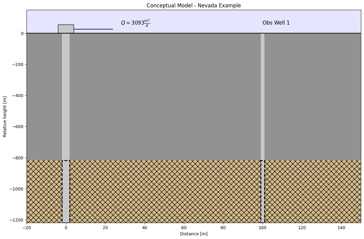
The example is taken from Kruseman and de Ridder (1990). It is based on a pumping test conducted in a fractured tertiary volcanic aquifer near Yucca Mountains, Nevada, US. Although conventional Darcy’s flow is not applied to fracture flow, in this case, we can assume that fracturing is pervasive enough to flow occur as Darcy’s flow at the aquifer scale. Flow to the well comes from fractures, while the matrix exchanges water with the fractures.
The borehole has 1219 m depth and penetrated a 400 m thick sequence of fractured volcanic rocks with water entry points. At every entry point, the head is more or less the same, so they have good hydraulic connection. The water table is about 470 m below depth, which indicates confined conditions.
Drawdown data was sampled at the well, named UE-25b#1 and at an observation well, named UE-25a#1, 110 m away. Three pumping tests were conducted at the site and will be the object of our investigation.
def conc_confined5():
    ##Now printing the conceptual model figure:

    fig = plt.figure(figsize=(14, 9))
    ax = fig.add_subplot(1, 1, 1)
    # sky
    sky = plt.Rectangle((-20, 0), width=170, height=150, fc="b", zorder=0, alpha=0.1)
    ax.add_patch(sky)

    # Aquifer:
    ground = plt.Rectangle(
        (-20, -1219),
        width=170,
        height=400,
        fc=np.array([209, 179, 127]) / 255,
        zorder=0,
        alpha=0.9,
        hatch="xx",
    )
    ax.add_patch(ground)

    # Confining bed:
    confining_unit = plt.Rectangle(
        (-20, -1219 + 400),
        width=170,
        height=1219 - 400,
        fc=np.array([100, 100, 100]) / 255,
        zorder=0,
        alpha=0.7,
    )
    ax.add_patch(confining_unit)
    well = plt.Rectangle(
        (-2, -1219), width=4, height=1219, fc=np.array([200, 200, 200]) / 255, zorder=1
    )
    ax.add_patch(well)

    # Wellhead
    wellhead = plt.Rectangle(
        (-4, 0),
        width=8,
        height=55,
        fc=np.array([200, 200, 200]) / 255,
        zorder=2,
        ec="k",
    )
    ax.add_patch(wellhead)

    # Screen for the well:
    screen = plt.Rectangle(
        (-2, -1219),
        width=4,
        height=400,
        fc=np.array([200, 200, 200]) / 255,
        alpha=1,
        zorder=2,
        ec="k",
        ls="--",
    )
    screen.set_linewidth(2)
    ax.add_patch(screen)
    pumping_arrow = plt.Arrow(x=4, y=25, dx=20, dy=0, color="#00035b", zorder=3)
    ax.add_patch(pumping_arrow)
    ax.text(x=28, y=55, s=r"$ Q = 3093 \frac{m^3}{d}$", fontsize="large")
    # Piezometers
    piez1 = plt.Rectangle(
        (99, -1219), width=2, height=1219, fc=np.array([200, 200, 200]) / 255, zorder=1
    )
    screen_piez_1 = plt.Rectangle(
        (99, -1219),
        width=2,
        height=400,
        fc=np.array([200, 200, 200]) / 255,
        alpha=1,
        zorder=2,
        ec="k",
        ls="--",
    )
    screen_piez_1.set_linewidth(2)

    ax.add_patch(piez1)

    ax.add_patch(screen_piez_1)

    # last line
    line = plt.Line2D(xdata=[-20, 150], ydata=[0, 0], color="k")
    ax.add_line(line)
    ax.text(x=100, y=55, s="Obs Well 1", fontsize="large")

    ax.set_xlim([-20, 150])
    ax.set_ylim([-1219, 150])
    ax.set_xlabel("Distance [m]")
    ax.set_ylabel("Relative height [m]")
    ax.set_title("Conceptual Model - Nevada Example")


conc_confined5()
Step 1. Import the Required Libraries#
import pandas as pd

import ttim
Step 2. Set the Basic Parameters for the Model#
H = 400  # aquifer thickness [m]
Q = 3093.12  # constant pumping rate [m^3/d]
Step 3. Load Data#
Dataset is stored in a text-file for each well, where the first column is the time in days and the second is the drawdown in meters.
# Pumped well UE-25b#1
data1 = np.loadtxt("data/double-porosity-pumpingwell.txt", skiprows=1)
t1 = data1[:, 0]
h1 = data1[:, 1]

# Observation well UE-25a#1
data2 = np.loadtxt("data/double-porosity-110m.txt", skiprows=1)
t2 = data2[:, 0]
h2 = data2[:, 1]
r = 110  # distance from obs to pumped well
Step 4. Create conceptual model#
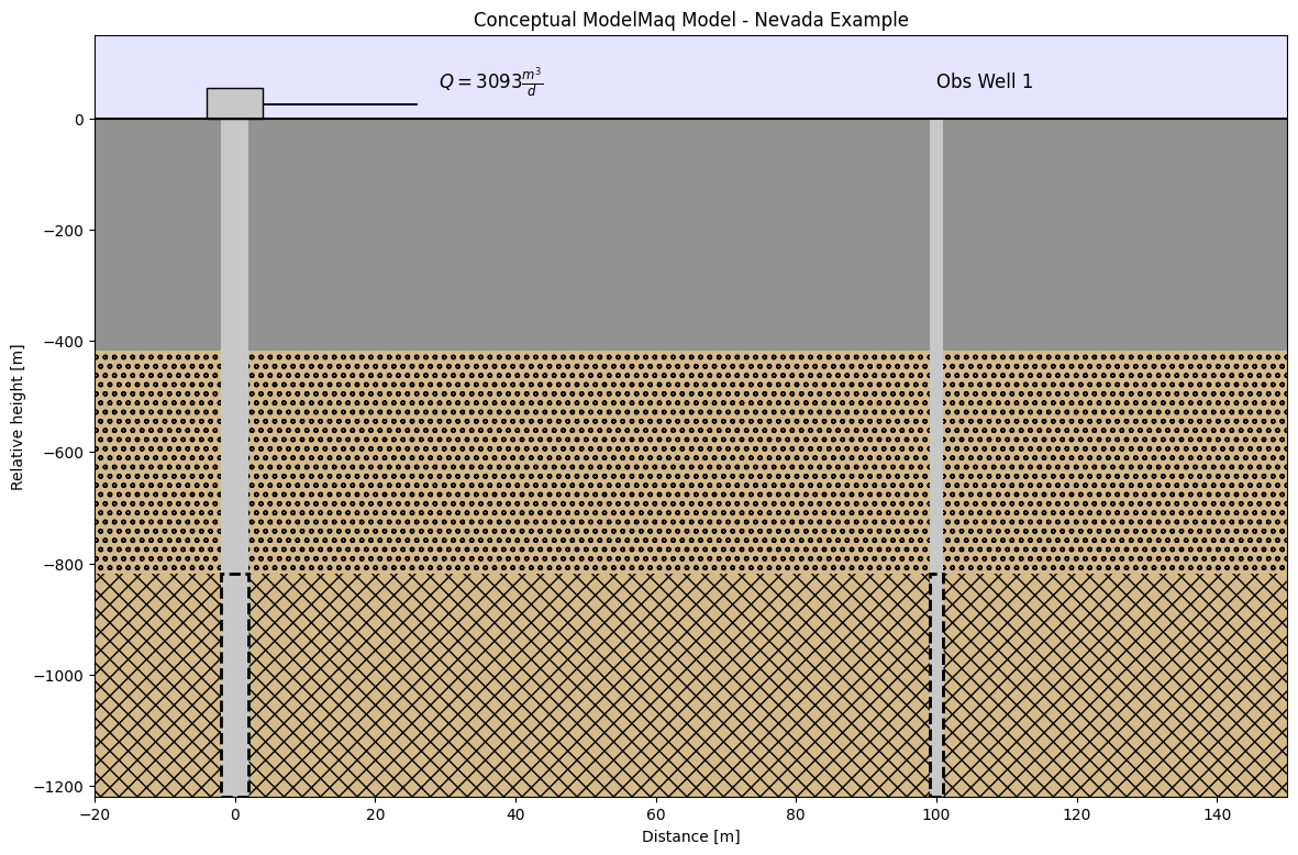
To conceptualize the model in TTim, we have to approximate the fractured system to a possible ModelMaq configuration. We can do this by creating a first layer that represents the matrix of the aquifer, followed by a 1 m thick aquitard and a second layer that represents the fractures.
def conc_mmaq_confined5():
    ##Now printing the conceptual model figure:

    fig = plt.figure(figsize=(14, 9))
    ax = fig.add_subplot(1, 1, 1)
    # sky
    sky = plt.Rectangle((-20, 0), width=170, height=150, fc="b", zorder=0, alpha=0.1)
    ax.add_patch(sky)

    # Aquifer:
    ground_2 = plt.Rectangle(
        (-20, -1219 + 401),
        width=170,
        height=400,
        fc=np.array([209, 179, 127]) / 255,
        zorder=0,
        alpha=0.9,
        hatch="oo",
    )
    ax.add_patch(ground_2)
    ground = plt.Rectangle(
        (-20, -1219),
        width=170,
        height=400,
        fc=np.array([209, 179, 127]) / 255,
        zorder=0,
        alpha=0.9,
        hatch="xx",
    )
    ax.add_patch(ground)

    # Confining bed:
    confining_unit_1 = plt.Rectangle(
        (-20, -1219 + 400),
        width=170,
        height=1,
        fc=np.array([100, 100, 100]) / 255,
        zorder=0,
        alpha=0.7,
    )
    ax.add_patch(confining_unit_1)
    confining_unit = plt.Rectangle(
        (-20, -1219 + 801),
        width=170,
        height=1219 - 801,
        fc=np.array([100, 100, 100]) / 255,
        zorder=0,
        alpha=0.7,
    )
    ax.add_patch(confining_unit)
    well = plt.Rectangle(
        (-2, -1219), width=4, height=1219, fc=np.array([200, 200, 200]) / 255, zorder=1
    )
    ax.add_patch(well)

    # Wellhead
    wellhead = plt.Rectangle(
        (-4, 0),
        width=8,
        height=55,
        fc=np.array([200, 200, 200]) / 255,
        zorder=2,
        ec="k",
    )
    ax.add_patch(wellhead)

    # Screen for the well:
    screen = plt.Rectangle(
        (-2, -1219),
        width=4,
        height=400,
        fc=np.array([200, 200, 200]) / 255,
        alpha=1,
        zorder=2,
        ec="k",
        ls="--",
    )
    screen.set_linewidth(2)
    ax.add_patch(screen)
    pumping_arrow = plt.Arrow(x=4, y=25, dx=22, dy=0, color="#00035b")
    ax.add_patch(pumping_arrow)
    ax.text(x=29, y=55, s=r"$ Q = 3093 \frac{m^3}{d}$", fontsize="large")
    # Piezometers
    piez1 = plt.Rectangle(
        (99, -1219), width=2, height=1219, fc=np.array([200, 200, 200]) / 255, zorder=1
    )
    screen_piez_1 = plt.Rectangle(
        (99, -1219),
        width=2,
        height=400,
        fc=np.array([200, 200, 200]) / 255,
        alpha=1,
        zorder=2,
        ec="k",
        ls="--",
    )
    screen_piez_1.set_linewidth(2)

    ax.add_patch(piez1)

    ax.add_patch(screen_piez_1)

    # last line
    line = plt.Line2D(xdata=[-20, 150], ydata=[0, 0], color="k")
    ax.add_line(line)
    ax.text(x=100, y=55, s="Obs Well 1", fontsize="large")

    ax.set_xlim([-20, 150])
    ax.set_ylim([-1219, 150])
    ax.set_xlabel("Distance [m]")
    ax.set_ylabel("Relative height [m]")
    ax.set_title("Conceptual ModelMaq Model - Nevada Example")
    plt.show()


conc_mmaq_confined5()
First, for the TTim model, we will adopt the parameters for the first layer from the results obtained from Kruseman and de Ridder (1970):
km = 0.1 / H  # hydraulic conductivity of matrix calculated by K&dR
Sm = 3.85e-4  # specific storage of matrix calculated by K&dR
Now we can construct the two-layer model: Instructions on how to construct this model are in:
ml = ttim.ModelMaq(
    kaq=[km, 1],
    z=[0, -400, -401, -801],
    c=5,
    Saq=[Sm, 1e-3],
    Sll=0,
    topboundary="conf",
    tmin=1e-5,
    tmax=3,
)
w = ttim.Well(ml, xw=0, yw=0, rw=0.11, rc=0, tsandQ=[0, 3093.12], layers=1)
ml.solve()
self.neq  1
solution complete
Step 5. Calibrate the model using both Datasets#
In this calibration procedure, we only calibrate the parameters of the fractured system and keep the matrix values fixed. We also calibrate the wellbore storage parameter rc that is the radius of the caisson considered for storage.
Instructions on how to set this calibration are in the notebook: Confined 1 - Oude Korendijk
ca = ttim.Calibrate(ml)
ca.set_parameter(name="kaq1", initial=10)
ca.set_parameter(name="Saq1", initial=1e-4, pmin=0)
ca.set_parameter(name="c1", initial=10)
ca.set_parameter_by_reference(name="rc", parameter=w.rc, initial=0)
ca.series(name="UE-25b#1", x=0, y=0, t=t1, h=h1, layer=1)
ca.series(name="UE-25a#1", x=r, y=0, t=t2, h=h2, layer=1)
ca.fit(report=True)
display(ca.parameters)
print("RMSE:", ca.rmse())
....................
......................
......................
......................
......................
......................
......................
......................
......................
...
Fit succeeded.
[[Fit Statistics]]
    # fitting method   = leastsq
    # function evals   = 196
    # data points      = 138
    # variables        = 4
    chi-square         = 5.47351756
    reduced chi-square = 0.04084715
    Akaike info crit   = -437.371845
    Bayesian info crit = -425.662830
[[Variables]]
    kaq1_1_1:  0.87696919 +/- 0.00699037 (0.80%) (init = 10)
    Saq1_1_1:  5.0874e-06 +/- 5.0674e-07 (9.96%) (init = 0.0001)
    c1_1_1:    13.0049034 +/- 1.59735201 (12.28%) (init = 10)
    rc:        0.10560391 +/- 0.00320829 (3.04%) (init = 0)
[[Correlations]] (unreported correlations are < 0.100)
    C(kaq1_1_1, c1_1_1)   = +0.8580
    C(kaq1_1_1, Saq1_1_1) = -0.7312
    C(Saq1_1_1, c1_1_1)   = -0.5463
    C(Saq1_1_1, rc)       = -0.4012
    C(kaq1_1_1, rc)       = +0.1007
RMSE: 0.19915614665911038
/tmp/ipykernel_1221/1053867569.py:2: DeprecationWarning: Setting layers in the parameter name is deprecated. Set the layers= keyword argument for parameter 'kaq1' to silence this warning. The parameter name can still include layer info, but this will be ignored in a future version of TTim.
  ca.set_parameter(name="kaq1", initial=10)
/tmp/ipykernel_1221/1053867569.py:3: DeprecationWarning: Setting layers in the parameter name is deprecated. Set the layers= keyword argument for parameter 'Saq1' to silence this warning. The parameter name can still include layer info, but this will be ignored in a future version of TTim.
  ca.set_parameter(name="Saq1", initial=1e-4, pmin=0)
/tmp/ipykernel_1221/1053867569.py:4: DeprecationWarning: Setting layers in the parameter name is deprecated. Set the layers= keyword argument for parameter 'c1' to silence this warning. The parameter name can still include layer info, but this will be ignored in a future version of TTim.
  ca.set_parameter(name="c1", initial=10)
| layers | optimal | std | perc_std | pmin | pmax | initial | inhoms | parray | |
|---|---|---|---|---|---|---|---|---|---|
| kaq1_1_1 | None | 0.876969 | 6.990369e-03 | 0.797105 | -inf | inf | 10.0000 | None | [[0.8769691909275003]] |
| Saq1_1_1 | None | 0.000005 | 5.067382e-07 | 9.960653 | 0.0 | inf | 0.0001 | None | [[5.0873991377375916e-06]] |
| c1_1_1 | None | 13.004903 | 1.597352e+00 | 12.282690 | -inf | inf | 10.0000 | None | [[13.00490342903561]] |
| rc | NaN | 0.105604 | 3.208291e-03 | 3.038042 | -inf | inf | 0.0000 | NaN | [[0.10560391385923244]] |
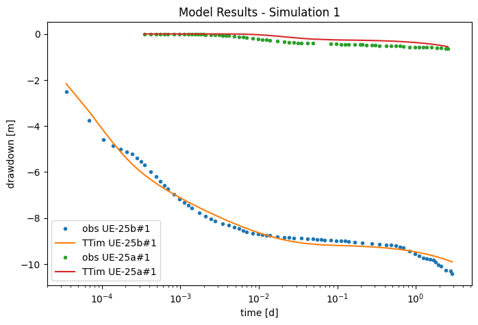
Overall, a good fit has been obtained. Reasonable standard deviations of the estimates and a low value for AIC and BIC gives us confidence in the adopted parameters. Now we can check how the results plot with the observations:
hm1 = ml.head(0, 0, t1)
hm2 = ml.head(110, 0, t2)
plt.figure(figsize=(8, 5))
plt.semilogx(t1, h1, ".", label="obs UE-25b#1")
plt.semilogx(t1, hm1[-1], label="TTim UE-25b#1")
plt.semilogx(t2, h2, ".", label="obs UE-25a#1")
plt.semilogx(t2, hm2[-1], label="TTim UE-25a#1")
plt.xlabel("time [d]")
plt.ylabel("drawdown [m]")
plt.title("Model Results - Simulation 1")
plt.legend();
Step 7. Simulate parameters of both fracture and matrix#
Now we will repeat the procedures of steps 5 and 6, but this time we will let TTim find the parameters for both the matrix and the fractures
ml1 = ttim.ModelMaq(
    kaq=[1, 1],
    z=[0, -400, -401, -801],
    c=5,
    Saq=[1e-3, 1e-3],
    Sll=0,
    topboundary="conf",
    tmin=1e-5,
    tmax=3,
)
w1 = ttim.Well(ml1, xw=0, yw=0, rw=0.11, rc=0, tsandQ=[0, 3093.12], layers=1)
ml1.solve()
self.neq  1
solution complete
ca1 = ttim.Calibrate(ml1)
ca1.set_parameter(name="kaq0", initial=1, pmin=1e-8)
ca1.set_parameter(name="Saq0", initial=1e-4, pmin=1e-8)
ca1.set_parameter(name="kaq1", initial=1, pmin=1e-8)
ca1.set_parameter(name="Saq1", initial=1e-4, pmin=1e-8)
ca1.set_parameter(name="c1", initial=100, pmin=1e-8)
ca1.set_parameter_by_reference(name="rc", parameter=w1.rc, initial=0, pmin=0)
ca1.series(name="UE-25b#1", x=0, y=0, t=t1, h=h1, layer=1)
ca1.series(name="UE-25a#1", x=110, y=0, t=t2, h=h2, layer=1)
ca1.fit(report=True)
display(ca1.parameters)
print("RMSE:", ca1.rmse())
....................
..
....................
..
....................
..
....................
..
....................
..
....................
..
....................
..
....................
..
....................
..
....................
..
....................
..
....................
..
....................
..
....................
..
....................
..
....................
..
....
Fit succeeded.
[[Fit Statistics]]
    # fitting method   = leastsq
    # function evals   = 353
    # data points      = 138
    # variables        = 6
    chi-square         = 3.51051320
    reduced chi-square = 0.02659480
    Akaike info crit   = -494.665820
    Bayesian info crit = -477.102298
[[Variables]]
    kaq0_0_0:  1.0900e-08 +/- 4.2595e-07 (3907.90%) (init = 1)
    Saq0_0_0:  1.4689e-04 +/- 1.4989e-05 (10.20%) (init = 0.0001)
    kaq1_1_1:  0.90737035 +/- 0.00606602 (0.67%) (init = 1)
    Saq1_1_1:  3.4662e-06 +/- 3.1083e-07 (8.97%) (init = 0.0001)
    c1_1_1:    15.2676476 +/- 1.42341377 (9.32%) (init = 100)
    rc:        0.10830776 +/- 0.00254979 (2.35%) (init = 0)
[[Correlations]] (unreported correlations are < 0.100)
    C(kaq1_1_1, Saq1_1_1) = -0.7404
    C(kaq1_1_1, c1_1_1)   = +0.7134
    C(Saq0_0_0, kaq1_1_1) = -0.6755
    C(Saq0_0_0, Saq1_1_1) = +0.5515
    C(Saq1_1_1, rc)       = -0.4148
    C(Saq1_1_1, c1_1_1)   = -0.3777
    C(Saq0_0_0, c1_1_1)   = -0.2750
    C(kaq0_0_0, c1_1_1)   = +0.1810
    C(kaq0_0_0, Saq1_1_1) = +0.1386
    C(kaq0_0_0, Saq0_0_0) = +0.1253
    C(kaq1_1_1, rc)       = +0.1180
    C(Saq0_0_0, rc)       = -0.1141
RMSE: 0.15949451851508745
/tmp/ipykernel_1221/3324531022.py:2: DeprecationWarning: Setting layers in the parameter name is deprecated. Set the layers= keyword argument for parameter 'kaq0' to silence this warning. The parameter name can still include layer info, but this will be ignored in a future version of TTim.
  ca1.set_parameter(name="kaq0", initial=1, pmin=1e-8)
/tmp/ipykernel_1221/3324531022.py:3: DeprecationWarning: Setting layers in the parameter name is deprecated. Set the layers= keyword argument for parameter 'Saq0' to silence this warning. The parameter name can still include layer info, but this will be ignored in a future version of TTim.
  ca1.set_parameter(name="Saq0", initial=1e-4, pmin=1e-8)
/tmp/ipykernel_1221/3324531022.py:4: DeprecationWarning: Setting layers in the parameter name is deprecated. Set the layers= keyword argument for parameter 'kaq1' to silence this warning. The parameter name can still include layer info, but this will be ignored in a future version of TTim.
  ca1.set_parameter(name="kaq1", initial=1, pmin=1e-8)
/tmp/ipykernel_1221/3324531022.py:5: DeprecationWarning: Setting layers in the parameter name is deprecated. Set the layers= keyword argument for parameter 'Saq1' to silence this warning. The parameter name can still include layer info, but this will be ignored in a future version of TTim.
  ca1.set_parameter(name="Saq1", initial=1e-4, pmin=1e-8)
/tmp/ipykernel_1221/3324531022.py:6: DeprecationWarning: Setting layers in the parameter name is deprecated. Set the layers= keyword argument for parameter 'c1' to silence this warning. The parameter name can still include layer info, but this will be ignored in a future version of TTim.
  ca1.set_parameter(name="c1", initial=100, pmin=1e-8)
/home/docs/checkouts/readthedocs.org/user_builds/ttim/envs/stable/lib/python3.11/site-packages/ttim/well.py:63: RuntimeWarning: divide by zero encountered in divide
  laboverrwk1 = self.aq.lab / (self.rw * kv(1, self.rw / self.aq.lab))
/home/docs/checkouts/readthedocs.org/user_builds/ttim/envs/stable/lib/python3.11/site-packages/ttim/well.py:63: RuntimeWarning: invalid value encountered in divide
  laboverrwk1 = self.aq.lab / (self.rw * kv(1, self.rw / self.aq.lab))
/home/docs/checkouts/readthedocs.org/user_builds/ttim/envs/stable/lib/python3.11/site-packages/ttim/well.py:66: RuntimeWarning: invalid value encountered in multiply
  self.term = -1.0 / (2 * np.pi) * laboverrwk1 * self.flowcoef * coef
| layers | optimal | std | perc_std | pmin | pmax | initial | inhoms | parray | |
|---|---|---|---|---|---|---|---|---|---|
| kaq0_0_0 | None | 1.089974e-08 | 4.259511e-07 | 3907.900289 | 1.000000e-08 | inf | 1.0000 | None | [[1.0899742997061423e-08]] |
| Saq0_0_0 | None | 1.468905e-04 | 1.498895e-05 | 10.204170 | 1.000000e-08 | inf | 0.0001 | None | [[0.0001468904856564146]] |
| kaq1_1_1 | None | 9.073704e-01 | 6.066017e-03 | 0.668527 | 1.000000e-08 | inf | 1.0000 | None | [[0.9073703507964265]] |
| Saq1_1_1 | None | 3.466185e-06 | 3.108291e-07 | 8.967469 | 1.000000e-08 | inf | 0.0001 | None | [[3.4661847544414925e-06]] |
| c1_1_1 | None | 1.526765e+01 | 1.423414e+00 | 9.323072 | 1.000000e-08 | inf | 100.0000 | None | [[15.267647615733086]] |
| rc | NaN | 1.083078e-01 | 2.549791e-03 | 2.354209 | 0.000000e+00 | inf | 0.0000 | NaN | [[0.10830775513910806]] |
We see that the fit has slightly improved, as the AIC and BIC values. However, from the table above, one can see that we have low confidence in the hydraulic conductivity of the matrix. Nevertheless, we can see it is a small value.
ht1 = ml1.head(0, 0, t1)
ht2 = ml1.head(110, 0, t2)
plt.figure(figsize=(8, 5))
plt.semilogx(t1, h1, ".", label="obs UE-25b#1")
plt.semilogx(t1, ht1[-1], label="TTim UE-25b#1")
plt.semilogx(t2, h2, ".", label="obs UE-25a#1")
plt.semilogx(t2, ht2[-1], label="TTim UE-25a#1")
plt.xlabel("time [d]")
plt.ylabel("drawdown [m]")
plt.title("Model Results - Simulation 1")
plt.legend()
plt.show()
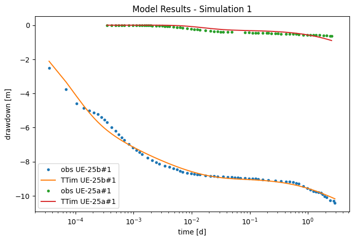
Overall the curves follow the trends of the drawdown and the fit is good in general.
Step 8. Analysis and Comparison of the Results under different methods#
The final important step is to compare the data obtained from this model with the data from other Aquifer Analysis software. Yang (2020) compared TTim results with the published results in Kruseman and de Ridder (1990), here abbreviated to K&dR, and with the results obtained from the software AQTESOLV (Duffield, 2007) and MLU (Carlson & Randall, 2012).
Kruseman et al. (1970) solved the problem using a graphical method, where the transmissivity was calculated as one aquifer and the storativity was separated between matrix and fractures. The MLU (Carlson & Randall, 2012) solution used a similar approach to our TTim model by simulating the matrix as a very-low transmissivity aquifer on top of the fractured aquifer and separated by a zero-storage aquitard. Yang (2020) solved the problem in AQTESOLV using a double-porosity analytical solution proposed by Moench (1984).
t = pd.DataFrame(
    columns=["km [m/d]", "Sm [1/m]", "kf [m/d]", "Sf [1/m]", "c", "rc"],
    index=[
        "K&dR",  #'Moench',
        "AQTESOLV",
        "MLU",
        "TTim1",
        "TTim2",
    ],
)
t.loc["TTim1"] = np.concatenate(
    (np.array([0.00025, 3.850e-04]), ca.parameters["optimal"].values)
)
t.loc["TTim2"] = ca1.parameters["optimal"].values
t.loc["K&dR"] = [0.8325, 3.750e-4, 0.8325, 4.000e-6, "-", "-"]
# I don't know where these values for Moench come from:
# t.loc['Moench'] = [0.1728, 3.000e-4, 0.864, 1.500e-6, '-', '-']
t.loc["AQTESOLV"] = [0.149, 5.512e-4, 0.937, 5.533e-6, "-", 0.11]
t.loc["MLU"] = [0.00025, 3.850e-04, 0.874, 8.053e-6, 12.380, 0.1]
t["RMSE"] = ["-", 0.031736, 0.434638, ca.rmse(), ca1.rmse()]
t
/home/docs/checkouts/readthedocs.org/user_builds/ttim/envs/stable/lib/python3.11/site-packages/ttim/well.py:63: RuntimeWarning: divide by zero encountered in divide
  laboverrwk1 = self.aq.lab / (self.rw * kv(1, self.rw / self.aq.lab))
/home/docs/checkouts/readthedocs.org/user_builds/ttim/envs/stable/lib/python3.11/site-packages/ttim/well.py:63: RuntimeWarning: invalid value encountered in divide
  laboverrwk1 = self.aq.lab / (self.rw * kv(1, self.rw / self.aq.lab))
/home/docs/checkouts/readthedocs.org/user_builds/ttim/envs/stable/lib/python3.11/site-packages/ttim/well.py:66: RuntimeWarning: invalid value encountered in multiply
  self.term = -1.0 / (2 * np.pi) * laboverrwk1 * self.flowcoef * coef
| km [m/d] | Sm [1/m] | kf [m/d] | Sf [1/m] | c | rc | RMSE | |
|---|---|---|---|---|---|---|---|
| K&dR | 0.8325 | 0.000375 | 0.8325 | 0.000004 | - | - | - |
| AQTESOLV | 0.149 | 0.000551 | 0.937 | 0.000006 | - | 0.11 | 0.031736 |
| MLU | 0.00025 | 0.000385 | 0.874 | 0.000008 | 12.38 | 0.1 | 0.434638 |
| TTim1 | 0.00025 | 0.000385 | 0.876969 | 0.000005 | 13.004903 | 0.105604 | 0.199156 |
| TTim2 | 0.0 | 0.000147 | 0.90737 | 0.000003 | 15.267648 | 0.108308 | 0.159495 |
Overall, TTim model 1 showed similar results to MLU but with a slightly better fit. AQTESOLV obtained the best fit using Moench’s analytical solution.
Step 8.1. Comparison of estimates and model error#
# Preparing the DataFrame:
t1 = pd.DataFrame(
    columns=["kaq - opt -l1", "kaq - 95% -l1", "kaq - opt -l2", "kaq - 95% -l2"],
    index=["AQTESOLV", "MLU", "K&dR", "TTim - all params", "TTim - fixed upper"],
)
simulation = ["AQTESOLV", "MLU", "K&dR", "TTim - rc", "TTim - fixed upper"]
t1.loc["MLU"] = [0.00025, np.nan, 0.874, 1.221 * 1e-2 * 0.874]
t1.loc["KdR"] = [0.8325, np.nan, 0.8325, np.nan]
t1.loc["AQTESOLV"] = [0.149, 291.236 * 1e-2 * 0.149, 0.937, 1.946 * 1e-2 * 0.937]
t1.loc["TTim - fixed upper"] = [
    0.00025,
    np.nan,
    ca.parameters.loc["kaq1", "optimal"],
    2 * ca.parameters.loc["kaq1", "std"],
]
t1.loc["TTim - all params"] = [
    ca1.parameters.loc["kaq0", "optimal"],
    2 * ca1.parameters.loc["kaq0", "std"],
    ca1.parameters.loc["kaq1", "optimal"],
    2 * ca1.parameters.loc["kaq1", "std"],
]

# Plotting

# plt.figure(figsize = (10,7))
fig, ax = plt.subplots(2, 1, figsize=(10, 7), sharex=True)
ax[0].errorbar(
    x=t1.index,
    y=t1["kaq - opt -l1"],
    yerr=[t1["kaq - 95% -l1"], t1["kaq - 95% -l1"]],
    marker="o",
    linestyle="",
    markersize=12,
    label="aquifer matrix",
    color="red",
)
ax[0].legend()
ax[1].errorbar(
    x=t1.index,
    y=t1["kaq - opt -l2"],
    yerr=[t1["kaq - 95% -l2"], t1["kaq - 95% -l2"]],
    marker="o",
    linestyle="",
    markersize=12,
    label="fractures",
)

plt.legend()
plt.title("Error bar plot of calibrated hydraulic conductivities")
plt.ylabel("K [m/d]")
# plt.ylim([278,289])
plt.xlabel("Model")
---------------------------------------------------------------------------
KeyError                                  Traceback (most recent call last)
File ~/checkouts/readthedocs.org/user_builds/ttim/envs/stable/lib/python3.11/site-packages/pandas/core/indexes/base.py:3641, in Index.get_loc(self, key)
   3640 try:
-> 3641     return self._engine.get_loc(casted_key)
   3642 except KeyError as err:

File pandas/_libs/index.pyx:168, in pandas._libs.index.IndexEngine.get_loc()

File pandas/_libs/index.pyx:197, in pandas._libs.index.IndexEngine.get_loc()

File pandas/_libs/hashtable_class_helper.pxi:7668, in pandas._libs.hashtable.PyObjectHashTable.get_item()

File pandas/_libs/hashtable_class_helper.pxi:7676, in pandas._libs.hashtable.PyObjectHashTable.get_item()

KeyError: 'kaq1'

The above exception was the direct cause of the following exception:

KeyError                                  Traceback (most recent call last)
Cell In[15], line 13
      8 t1.loc["KdR"] = [0.8325, np.nan, 0.8325, np.nan]
      9 t1.loc["AQTESOLV"] = [0.149, 291.236 * 1e-2 * 0.149, 0.937, 1.946 * 1e-2 * 0.937]
     10 t1.loc["TTim - fixed upper"] = [
     11     0.00025,
     12     np.nan,
---> 13     ca.parameters.loc["kaq1", "optimal"],
     14     2 * ca.parameters.loc["kaq1", "std"],
     15 ]
     16 t1.loc["TTim - all params"] = [
     17     ca1.parameters.loc["kaq0", "optimal"],
     18     2 * ca1.parameters.loc["kaq0", "std"],
     19     ca1.parameters.loc["kaq1", "optimal"],
     20     2 * ca1.parameters.loc["kaq1", "std"],
     21 ]
     23 # Plotting
     24
     25 # plt.figure(figsize = (10,7))

File ~/checkouts/readthedocs.org/user_builds/ttim/envs/stable/lib/python3.11/site-packages/pandas/core/indexing.py:1199, in _LocationIndexer.__getitem__(self, key)
   1197     key = tuple(com.apply_if_callable(x, self.obj) for x in key)
   1198     if self._is_scalar_access(key):
-> 1199         return self.obj._get_value(*key, takeable=self._takeable)
   1200     return self._getitem_tuple(key)
   1201 else:
   1202     # we by definition only have the 0th axis

File ~/checkouts/readthedocs.org/user_builds/ttim/envs/stable/lib/python3.11/site-packages/pandas/core/frame.py:4495, in DataFrame._get_value(self, index, col, takeable)
   4489 series = self._get_item(col)
   4491 if not isinstance(self.index, MultiIndex):
   4492     # CategoricalIndex: Trying to use the engine fastpath may give incorrect
   4493     #  results if our categories are integers that dont match our codes
   4494     # IntervalIndex: IntervalTree has no get_loc
-> 4495     row = self.index.get_loc(index)
   4496     return series._values[row]
   4498 # For MultiIndex going through engine effectively restricts us to
   4499 #  same-length tuples; see test_get_set_value_no_partial_indexing

File ~/checkouts/readthedocs.org/user_builds/ttim/envs/stable/lib/python3.11/site-packages/pandas/core/indexes/base.py:3648, in Index.get_loc(self, key)
   3643     if isinstance(casted_key, slice) or (
   3644         isinstance(casted_key, abc.Iterable)
   3645         and any(isinstance(x, slice) for x in casted_key)
   3646     ):
   3647         raise InvalidIndexError(key) from err
-> 3648     raise KeyError(key) from err
   3649 except TypeError:
   3650     # If we have a listlike key, _check_indexing_error will raise
   3651     #  InvalidIndexError. Otherwise we fall through and re-raise
   3652     #  the TypeError.
   3653     self._check_indexing_error(key)

KeyError: 'kaq1'
Hydraulic conductivities varied between simulations. When estimated, the matrix conductivity had higher uncertainty. Uncertainty ranges are similar for the fractured portion. However, the solutions do not always overlap each other.
Reference#
Carlson F, Randall J (2012) MLU: a Windows application for the analysis of aquifer tests and the design of well fields in layered systems. Ground Water 50(4):504–510
Duffield, G.M., 2007. AQTESOLV for Windows Version 4.5 User’s Guide, HydroSOLVE, Inc., Reston, VA.
Kruseman GP, De Ridder NA (1990) Analysis and evaluation of pumping test data, 2nd edn. ILRI Publ. 47, ILRI, Wageningen, The Netherlands
Moench, A. F. (1984), Double-Porosity Models for a Fissured Groundwater Reservoir With Fracture Skin, Water Resour. Res., 20( 7), 831– 846, doi:10.1029/WR020i007p00831.
Yang, Xinzhu (2020) Application and comparison of different methodsfor aquifer test analysis using TTim. Master Thesis, Delft University of Technology (TUDelft), Delft, The Netherlands.