3. Confined Aquifer Test - Sioux Example#

This test is taken from AQTESOLV examples.

Introduction and Conceptual Model#

In this example, we reproduce the work of Yang (2020) to use the pumping test data to demonstrate how TTim can be used to model and analyze pumping tests in a single layer, confined setting, in multiple piezometers. Furthermore, we compare the performance of TTim with other transient well hydraulics software AQTESOLV (Duffield, 2007) and MLU (Carlson and Randall, 2012).

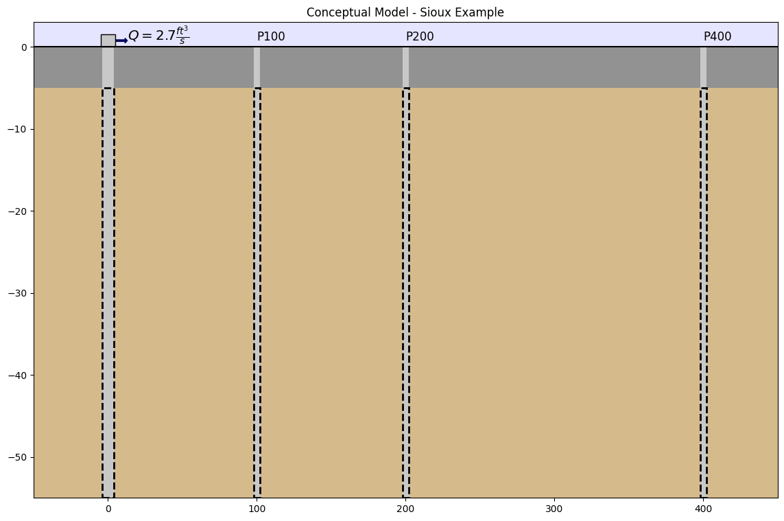
This example is a pumping test done in Sioux Flats, South Dakota, USA. The data comes from the AQTESOLV documentation (Duffield, 2007). The aquifer is 50 ft thick and is bounded by impermeable layers. The test was conducted for 2045 minutes (~34 hours), with a constant pumping rate of 2.7 \(ft^3/s\). Drawdown data has been collected at three piezometers located 100, 200 and 400 ft away, respectively. The well radius is 0.5 ft.

We can resume the conceptual model in the picture below:

Show code cell source

Hide code cell source

import matplotlib.pyplot as plt
import numpy as np

##Now printing the conceptual model figure:

fig = plt.figure(figsize=(14, 9))
ax = fig.add_subplot(1, 1, 1)
# sky
sky = plt.Rectangle((-50, 0), width=500, height=3, fc="b", zorder=0, alpha=0.1)
ax.add_patch(sky)

# Aquifer:
ground = plt.Rectangle(
    (-50, -55),
    width=500,
    height=50,
    fc=np.array([209, 179, 127]) / 255,
    zorder=0,
    alpha=0.9,
)
ax.add_patch(ground)

# Confining bed:
confining_unit = plt.Rectangle(
    (-50, -5),
    width=500,
    height=5,
    fc=np.array([100, 100, 100]) / 255,
    zorder=0,
    alpha=0.7,
)
ax.add_patch(confining_unit)
well = plt.Rectangle(
    (-4, -55), width=8, height=55, fc=np.array([200, 200, 200]) / 255, zorder=1
)
ax.add_patch(well)

# Wellhead
wellhead = plt.Rectangle(
    (-5, 0), width=10, height=1.5, fc=np.array([200, 200, 200]) / 255, zorder=2, ec="k"
)
ax.add_patch(wellhead)

# Screen for the well:
screen = plt.Rectangle(
    (-4, -55),
    width=8,
    height=50,
    fc=np.array([200, 200, 200]) / 255,
    alpha=1,
    zorder=2,
    ec="k",
    ls="--",
)
screen.set_linewidth(2)
ax.add_patch(screen)
pumping_arrow = plt.Arrow(x=5, y=0.75, dx=8, dy=0, color="#00035b")
ax.add_patch(pumping_arrow)
ax.text(x=13, y=0.75, s=r"$ Q = 2.7 \frac{ft^3}{s}$", fontsize="x-large")
# Piezometers
piez1 = plt.Rectangle(
    (98, -55), width=4, height=55, fc=np.array([200, 200, 200]) / 255, zorder=1
)
piez2 = plt.Rectangle(
    (198, -55), width=4, height=55, fc=np.array([200, 200, 200]) / 255, zorder=1
)
piez3 = plt.Rectangle(
    (398, -55), width=4, height=55, fc=np.array([200, 200, 200]) / 255, zorder=1
)

screen_piez_1 = plt.Rectangle(
    (98, -55),
    width=4,
    height=50,
    fc=np.array([200, 200, 200]) / 255,
    alpha=1,
    zorder=2,
    ec="k",
    ls="--",
)
screen_piez_1.set_linewidth(2)
screen_piez_2 = plt.Rectangle(
    (198, -55),
    width=4,
    height=50,
    fc=np.array([200, 200, 200]) / 255,
    alpha=1,
    zorder=2,
    ec="k",
    ls="--",
)
screen_piez_2.set_linewidth(2)
screen_piez_3 = plt.Rectangle(
    (398, -55),
    width=4,
    height=50,
    fc=np.array([200, 200, 200]) / 255,
    alpha=1,
    zorder=2,
    ec="k",
    ls="--",
)
screen_piez_3.set_linewidth(2)
ax.add_patch(piez1)
ax.add_patch(piez2)
ax.add_patch(piez3)
ax.add_patch(screen_piez_1)
ax.add_patch(screen_piez_2)
ax.add_patch(screen_piez_3)
# last line
line = plt.Line2D(xdata=[-50, 500], ydata=[0, 0], color="k")
ax.add_line(line)
ax.text(x=100, y=0.75, s="P100", fontsize="large")
ax.text(x=200, y=0.75, s="P200", fontsize="large")
ax.text(x=400, y=0.75, s="P400", fontsize="large")
ax.set_xlim([-50, 450])
ax.set_ylim([-55, 3])
ax.set_title("Conceptual Model - Sioux Example");

../_images/119755d68ff0c62ba0d1262f1467974ae70f853d6f264ebf4f9f3104ac227ba3.png

Step 1. Load Required Libraries#

import matplotlib.pyplot as plt
import numpy as np
import pandas as pd

import ttim

Step 2. Set basic parameters#

We will work with time in days and length in meters from this step onwards
The parameters below have already been converted to m and days.

Q = 6605.754  # constant discharge in m^3/d
b = -15.24  # aquifer thickness in m
rw = 0.1524  # well radius in m
r1 = 30.48  # distance between obs1 to pumping well
r2 = 60.96  # distance between obs2 to pumping well
r3 = 121.92  # distance between obs3 to pumping well

Step 3. Load data of observation and pumping well#

The preferred method of loading data into TTim is to use numpy arrays.

The data is in a text file where the first column is the time data in days and the second column is the drawdown in meters

For each piezometer, we will load the data as a numpy array. We further split the data into two different 1d arrays, one for time and another for drawdown.

data1 = np.loadtxt("data/sioux100.txt")
t1 = data1[:, 0]
h1 = data1[:, 1]


data2 = np.loadtxt("data/sioux200.txt")
t2 = data2[:, 0]
h2 = data2[:, 1]

data3 = np.loadtxt("data/sioux400.txt")
t3 = data3[:, 0]
h3 = data3[:, 1]

Step 4. Creating a TTim conceptual model#

In this example, we are using the ModelMaq model to conceptualize our aquifer. ModelMaq defines the aquifer system as a stacked vertical sequence of aquifers and leaky layers (aquifer-leaky layer, aquifer-leaky layer, etc). A thorough explanation of the ModelMaq and TTim one-layer modelling conceptualization is given in the notebook: Confined 1 - Oude Korendijk

ml_0 = ttim.ModelMaq(kaq=10, z=[0, b], Saq=0.001, tmin=0.001, tmax=10, topboundary="conf")
w_0 = ttim.Well(ml_0, xw=0, yw=0, rw=rw, tsandQ=[(0, Q)], layers=0)
ml_0.solve()

self.neq  1
solution complete

Step 5. Calibration#

The calibration workflow has been described in detail in the notebook: Confined 1 - Oude Korendijk

Step 5.1. Model Calibration with all observation wells#

We calibrate the model with all observation wells. We begin by assuming no wellbore storage or skin resistance, and we only calibrate the hydraulic conductivity and specific storage

# unknown parameters: k, Saq
ca_0 = ttim.Calibrate(ml_0)
ca_0.set_parameter(name="kaq0", initial=10)
ca_0.set_parameter(name="Saq0", initial=1e-4)
ca_0.series(name="obs1", x=r1, y=0, t=t1, h=h1, layer=0)
ca_0.series(name="obs2", x=r2, y=0, t=t2, h=h2, layer=0)
ca_0.series(name="obs3", x=r3, y=0, t=t3, h=h3, layer=0)
ca_0.fit(report=True)

..................................
....
Fit succeeded.
[[Fit Statistics]]
    # fitting method   = leastsq
    # function evals   = 35
    # data points      = 77
    # variables        = 2
    chi-square         = 0.00121634
    reduced chi-square = 1.6218e-05
    Akaike info crit   = -847.289916
    Bayesian info crit = -842.602305
[[Variables]]
    kaq0_0_0:  282.795231 +/- 1.13788961 (0.40%) (init = 10)
    Saq0_0_0:  0.00420855 +/- 3.3461e-05 (0.80%) (init = 0.0001)
[[Correlations]] (unreported correlations are < 0.100)
    C(kaq0_0_0, Saq0_0_0) = -0.8113

/tmp/ipykernel_1166/3426715523.py:3: DeprecationWarning: Setting layers in the parameter name is deprecated. Set the layers= keyword argument for parameter 'kaq0' to silence this warning. The parameter name can still include layer info, but this will be ignored in a future version of TTim.
  ca_0.set_parameter(name="kaq0", initial=10)
/tmp/ipykernel_1166/3426715523.py:4: DeprecationWarning: Setting layers in the parameter name is deprecated. Set the layers= keyword argument for parameter 'Saq0' to silence this warning. The parameter name can still include layer info, but this will be ignored in a future version of TTim.
  ca_0.set_parameter(name="Saq0", initial=1e-4)

display(ca_0.parameters)
print("RMSE:", ca_0.rmse())

	layers	optimal	std	perc_std	pmin	pmax	initial	inhoms	parray
kaq0_0_0	None	282.795231	1.137890	0.402372	-inf	inf	10.0000	None	[[282.795230967009]]
Saq0_0_0	None	0.004209	0.000033	0.795066	-inf	inf	0.0001	None	[[0.004208547431334762]]

RMSE: 0.0039744989134253405

Model has achieved a good fit and parameters with a low confidence interval

hm1_0 = ml_0.head(x=r1, y=0, t=t1)
hm2_0 = ml_0.head(x=r2, y=0, t=t2)
hm3_0 = ml_0.head(x=r3, y=0, t=t3)
plt.figure(figsize=(10, 7))
plt.semilogx(t1, h1, ".", label="obs1")
plt.semilogx(t1, hm1_0[0], label="ttim result 1")
plt.semilogx(t2, h2, ".", label="obs2")
plt.semilogx(t2, hm2_0[0], label="ttim result 2")
plt.semilogx(t3, h3, ".", label="obs3")
plt.semilogx(t3, hm3_0[0], label="ttim result 3")
plt.xlabel("time [d]")
plt.ylabel("drawdown [m]")
plt.legend()
plt.title("Calibration Results vs Observations - Model 1");

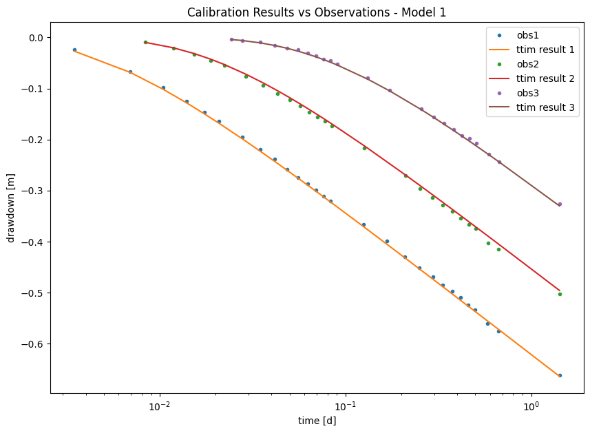
../_images/9dbb26b10948e69a0158d7b75c8925402d5a3c4cd59cb14e8aa811db4d0ad70f.png

Visually, the model seems to have a good fit with the data

Step 5.2. Model Calibration with wellbore storage#

In this new model, we investigate whether the well parameters are relevant in the fit.

We begin by reloading the model and creating a Well object with one extra parameters:

The radius of the caisson rc, which we use to simulate wellbore storage. In this case, we use a value in meters (float);

ml_1 = ttim.ModelMaq(kaq=10, z=[0, b], Saq=0.001, tmin=0.001, tmax=10, topboundary="conf")
w_1 = ttim.Well(ml_1, xw=0, yw=0, rw=rw, rc=0, tsandQ=[(0, Q)], layers=0)
ml_1.solve()

self.neq  1
solution complete

Here we use the method .set_parameter_by_reference to calibrate the rc parameter in our well.

.set_parameter_by_reference takes the following arguments:

name: a string of the parameter name
parameter: numpy-array with the parameter to be optimized. It should be specified as a reference, for example, in our case: w1.rc[0:] referencing to the parameter rc in object w1.
initial: float with the initial guess for the parameter value.
pmin and pmax: floats with the minimum and maximum values allowed. If not specified, these will be -np.inf and np.inf.

# unknown parameters: k, Saq, res, rc
ca_1 = ttim.Calibrate(ml_1)
ca_1.set_parameter(name="kaq0", initial=10)
ca_1.set_parameter(name="Saq0", initial=1e-4)
ca_1.set_parameter_by_reference(name="rc", parameter=w_1.rc, pmin=0.1, initial=0.2)
ca_1.series(name="obs1", x=r1, y=0, t=t1, h=h1, layer=0)
ca_1.series(name="obs2", x=r2, y=0, t=t2, h=h2, layer=0)
ca_1.series(name="obs3", x=r3, y=0, t=t3, h=h3, layer=0)
ca_1.fit(report=True)

..................................
..
...................
Fit succeeded.
[[Fit Statistics]]
    # fitting method   = leastsq
    # function evals   = 52
    # data points      = 77
    # variables        = 3
    chi-square         = 0.00116245
    reduced chi-square = 1.5709e-05
    Akaike info crit   = -848.779377
    Bayesian info crit = -841.747961
[[Variables]]
    kaq0_0_0:  283.922336 +/- 1.28527851 (0.45%) (init = 10)
    Saq0_0_0:  0.00415478 +/- 4.3879e-05 (1.06%) (init = 0.0001)
    rc:        0.78994252 +/- 0.21182305 (26.81%) (init = 0.2)
[[Correlations]] (unreported correlations are < 0.100)
    C(kaq0_0_0, Saq0_0_0) = -0.8522
    C(Saq0_0_0, rc)       = -0.6690
    C(kaq0_0_0, rc)       = +0.4874

/tmp/ipykernel_1166/3986394332.py:3: DeprecationWarning: Setting layers in the parameter name is deprecated. Set the layers= keyword argument for parameter 'kaq0' to silence this warning. The parameter name can still include layer info, but this will be ignored in a future version of TTim.
  ca_1.set_parameter(name="kaq0", initial=10)
/tmp/ipykernel_1166/3986394332.py:4: DeprecationWarning: Setting layers in the parameter name is deprecated. Set the layers= keyword argument for parameter 'Saq0' to silence this warning. The parameter name can still include layer info, but this will be ignored in a future version of TTim.
  ca_1.set_parameter(name="Saq0", initial=1e-4)

display(ca_1.parameters)
print("RMSE:", ca_1.rmse())

	layers	optimal	std	perc_std	pmin	pmax	initial	inhoms	parray
kaq0_0_0	None	283.922336	1.285279	0.452687	-inf	inf	10.0000	None	[[283.9223355922269]]
Saq0_0_0	None	0.004155	0.000044	1.056101	-inf	inf	0.0001	None	[[0.0041547806676629235]]
rc	NaN	0.789943	0.211823	26.814995	0.1	inf	0.2000	NaN	[[0.7899425195211106]]

RMSE: 0.003885454027411197

The new model has better statistics: lower AIC and BIC, lower RMSE and lower standard deviations for hydraulic conductivities and specific storage. We proceed with plotting the results:

hm1_1 = ml_1.head(r1, 0, t1)
hm2_1 = ml_1.head(r2, 0, t2)
hm3_1 = ml_1.head(r3, 0, t3)
plt.figure(figsize=(10, 7))
plt.semilogx(t1, h1, ".", label="obs1")
plt.semilogx(t1, hm1_1[0], label="ttim1")
plt.semilogx(t2, h2, ".", label="obs2")
plt.semilogx(t2, hm2_1[0], label="ttim2")
plt.semilogx(t3, h3, ".", label="obs3")
plt.semilogx(t3, hm3_1[0], label="ttim3")
plt.xlabel("time [d]")
plt.ylabel("drawdown [m]")
plt.legend()
plt.title("Model Calibration Results - Model 2");

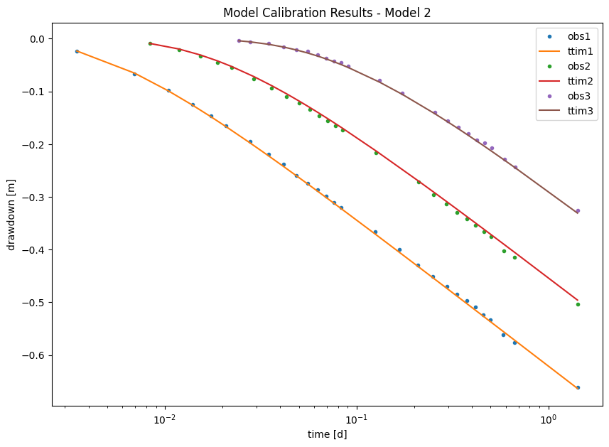
../_images/6662b88fc70cc8e5365e8f4fba9ebdade09c8c8aa90ac9ca9b70c81e6d1481f4.png

From the plot above, we can see that there is good agreement between the model calculated heads and the observed ones for all observation wells

Step 6. Analysis of Results#

Step 6.1. Analysis of Fit Statistics#

Some of the fit statistics are stored in the fitresult attribute of the calibration object. This object is a lmfit MinimizerResult object. lmfit is the python library doing the calibration for TTim behind the scenes. We accessed below the AIC and BIC values of this object.

Check the lmfit documentation (Newville et al. 2014) to learn more about this object and lmfit.

t = pd.DataFrame(
    columns=["RMSE", "AIC", "BIC", "Calibration scheme"], index=["Model 1", "Model 2"]
)

t["RMSE"] = [ca_0.rmse(), ca_1.rmse()]

t["AIC"] = [ca_0.fitresult.aic, ca_1.fitresult.aic]

t["BIC"] = [ca_0.fitresult.bic, ca_1.fitresult.bic]

t["Calibration scheme"] = ["All Obs Wells", "All Obs Wells + wellbore storage"]
t.style.set_caption("Fit statistics for the tested models")

Fit statistics for the tested models
	RMSE	AIC	BIC	Calibration scheme
Model 1	0.003974	-847.289916	-842.602305	All Obs Wells
Model 2	0.003885	-848.779377	-841.747961	All Obs Wells + wellbore storage

The fit statistics show that the models have very similar performance as all indicators are closely related. By RMSE and AIC criteria, we should pick Model 2, while by BIC, we should pick Model 1. The result means that we cannot exclude one model in favour of the other.

Step 6.2. Summary of Calibrated Parameters and comparison with different Software solutions#

We present the results simulated in TTim under different configurations below. Furthermore, Yang (2020) compared TTim results with the results obtained from the software AQTESOLV (Duffield, 2007) and MLU (Carlson & Randall, 2012). In both software, the model was calibrated with observations.

t = pd.DataFrame(
    columns=["k [m/d]", "Ss [1/m]", "rc"], index=["AQTESOLV", "MLU", "ttim", "ttim-rc"]
)
t.loc["AQTESOLV"] = [282.659, 4.211e-03, "-"]
t.loc["ttim"] = np.append(ca_0.parameters["optimal"].values, "-")
t.loc["ttim-rc"] = ca_1.parameters["optimal"].values
t.loc["MLU"] = [282.684, 4.209e-03, "-"]
t["RMSE"] = [0.003925, 0.003897, ca_0.rmse(), ca_1.rmse()]
t

	k [m/d]	Ss [1/m]	rc	RMSE
AQTESOLV	282.659	0.004211	-	0.003925
MLU	282.684	0.004209	-	0.003897
ttim	282.795230967009	0.004208547431334762	-	0.003974
ttim-rc	283.922336	0.004155	0.789943	0.003885

TTim achieved similar results with the other software. The TTim model with wellbore storage had a slightly better RMSE error.

# Preparing the DataFrame:
t1 = pd.DataFrame(
    columns=["kaq - opt", "kaq - 95%"], index=["MLU", "AQTESOLV", "TTim", "TTim - rc"]
)
simulation = ["MLU", "AQTESOLV", "TTim", "TTim - rc"]
t1.loc["MLU"] = [282.684, 0.783 * 1e-2 * 282.6842]
t1.loc["AQTESOLV"] = [282.659, 0.394 * 1e-2 * 282.659]
t1.loc["TTim"] = [
    ca_0.parameters.loc["kaq0", "optimal"],
    2 * ca_0.parameters.loc["kaq0", "std"],
]
t1.loc["TTim - rc"] = [
    ca_1.parameters.loc["kaq0", "optimal"],
    2 * ca_0.parameters.loc["kaq0", "std"],
]

# Plotting

plt.figure(figsize=(10, 7))

plt.errorbar(
    x=t1.index,
    y=t1["kaq - opt"],
    yerr=[t1["kaq - 95%"], t1["kaq - 95%"]],
    marker="o",
    linestyle="",
    markersize=12,
)
# plt.legend()
plt.title("Error bar plot of calibrated hydraulic conductivities")
plt.ylabel("K [m/d]")
plt.ylim([278, 289])
plt.xlabel("Model");

---------------------------------------------------------------------------
KeyError                                  Traceback (most recent call last)
File ~/checkouts/readthedocs.org/user_builds/ttim/envs/stable/lib/python3.11/site-packages/pandas/core/indexes/base.py:3641, in Index.get_loc(self, key)
   3640 try:
-> 3641     return self._engine.get_loc(casted_key)
   3642 except KeyError as err:

File pandas/_libs/index.pyx:168, in pandas._libs.index.IndexEngine.get_loc()

File pandas/_libs/index.pyx:197, in pandas._libs.index.IndexEngine.get_loc()

File pandas/_libs/hashtable_class_helper.pxi:7668, in pandas._libs.hashtable.PyObjectHashTable.get_item()

File pandas/_libs/hashtable_class_helper.pxi:7676, in pandas._libs.hashtable.PyObjectHashTable.get_item()

KeyError: 'kaq0'

The above exception was the direct cause of the following exception:

KeyError                                  Traceback (most recent call last)
Cell In[15], line 9
      6 t1.loc["MLU"] = [282.684, 0.783 * 1e-2 * 282.6842]
      7 t1.loc["AQTESOLV"] = [282.659, 0.394 * 1e-2 * 282.659]
      8 t1.loc["TTim"] = [
----> 9     ca_0.parameters.loc["kaq0", "optimal"],
     10     2 * ca_0.parameters.loc["kaq0", "std"],
     11 ]
     12 t1.loc["TTim - rc"] = [
     13     ca_1.parameters.loc["kaq0", "optimal"],
     14     2 * ca_0.parameters.loc["kaq0", "std"],
     15 ]
     17 # Plotting

File ~/checkouts/readthedocs.org/user_builds/ttim/envs/stable/lib/python3.11/site-packages/pandas/core/indexing.py:1199, in _LocationIndexer.__getitem__(self, key)
   1197     key = tuple(com.apply_if_callable(x, self.obj) for x in key)
   1198     if self._is_scalar_access(key):
-> 1199         return self.obj._get_value(*key, takeable=self._takeable)
   1200     return self._getitem_tuple(key)
   1201 else:
   1202     # we by definition only have the 0th axis

File ~/checkouts/readthedocs.org/user_builds/ttim/envs/stable/lib/python3.11/site-packages/pandas/core/frame.py:4495, in DataFrame._get_value(self, index, col, takeable)
   4489 series = self._get_item(col)
   4491 if not isinstance(self.index, MultiIndex):
   4492     # CategoricalIndex: Trying to use the engine fastpath may give incorrect
   4493     #  results if our categories are integers that dont match our codes
   4494     # IntervalIndex: IntervalTree has no get_loc
-> 4495     row = self.index.get_loc(index)
   4496     return series._values[row]
   4498 # For MultiIndex going through engine effectively restricts us to
   4499 #  same-length tuples; see test_get_set_value_no_partial_indexing

File ~/checkouts/readthedocs.org/user_builds/ttim/envs/stable/lib/python3.11/site-packages/pandas/core/indexes/base.py:3648, in Index.get_loc(self, key)
   3643     if isinstance(casted_key, slice) or (
   3644         isinstance(casted_key, abc.Iterable)
   3645         and any(isinstance(x, slice) for x in casted_key)
   3646     ):
   3647         raise InvalidIndexError(key) from err
-> 3648     raise KeyError(key) from err
   3649 except TypeError:
   3650     # If we have a listlike key, _check_indexing_error will raise
   3651     #  InvalidIndexError. Otherwise we fall through and re-raise
   3652     #  the TypeError.
   3653     self._check_indexing_error(key)

KeyError: 'kaq0'

Error bar plot shows AQTESOLV with the lowest confidence interval. The models in TTim have larger confidence intervals. However, they are still small. All models seem to agree, and there is a wide overlap in the confidence intervals for hydraulic conductivity

References#

Carlson F, Randall J (2012) MLU: a Windows application for the analysis of aquifer tests and the design of well fields in layered systems. Ground Water 50(4):504–510
Duffield, G.M., 2007. AQTESOLV for Windows Version 4.5 User’s Guide, HydroSOLVE, Inc., Reston, VA.
Newville, M.,Stensitzki, T., Allen, D.B., Ingargiola, A. (2014) LMFIT: Non Linear Least-Squares Minimization and Curve Fitting for Python.https://dx.doi.org/10.5281/zenodo.11813. https://lmfit.github.io/lmfit-py/intro.html (last access: August,2021).
Yang, Xinzhu (2020) Application and comparison of different methodsfor aquifer test analysis using TTim. Master Thesis, Delft University of Technology (TUDelft), Delft, The Netherlands.