3. Synthetic Pumping Test - Calibration test

import matplotlib.pyplot as plt
import numpy as np

import ttim

Use observation times from Oude Korendijk

drawdown = np.loadtxt("data/oudekorendijk_h30.dat")
tobs = drawdown[:, 0] / 60 / 24
robs = 30
Q = 788

Generate data

ml = ttim.ModelMaq(kaq=60, z=(-18, -25), Saq=1e-4, tmin=1e-5, tmax=1)
w = ttim.Well(ml, xw=0, yw=0, rw=0.1, tsandQ=[(0, 788)], layers=0)
ml.solve()
rnd = np.random.default_rng(2)
hobs = ml.head(robs, 0, tobs)[0] + 0.05 * rnd.random(len(tobs))

self.neq  1
solution complete

See if TTim can find aquifer parameters back

cal = ttim.Calibrate(ml)
cal.set_parameter(name="kaq0", layers=0, initial=100)
cal.set_parameter(name="Saq0", layers=0, initial=1e-3)
cal.series(name="obs1", x=robs, y=0, layer=0, t=tobs, h=hobs)
cal.fit()

................................
....
Fit succeeded.

cal.parameters

	layers	optimal	std	perc_std	pmin	pmax	initial	inhoms	parray
kaq0_0_0	0	59.871358	0.670180	1.119366	-inf	inf	100.000	None	[[59.87135844623144]]
Saq0_0_0	0	0.000121	0.000004	3.633645	-inf	inf	0.001	None	[[0.00012118958795889718]]

print("rmse:", cal.rmse())

rmse: 0.014201293762177191

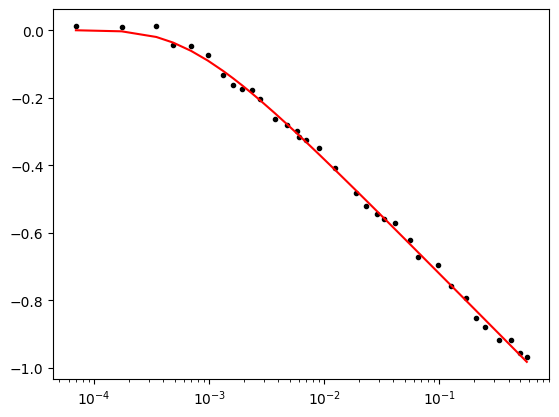
hm = ml.head(robs, 0, tobs, 0)
plt.semilogx(tobs, hobs, ".k")
plt.semilogx(tobs, hm[0], "r");

print("correlation matrix")
print(cal.fitresult.covar)

correlation matrix
[[ 4.49140659e-01 -2.49689444e-06]
 [-2.49689444e-06  1.93916877e-11]]

Fit with scipy.least_squares (not recommended)

cal = ttim.Calibrate(ml)
cal.set_parameter(name="kaq0", layers=0, initial=100)
cal.set_parameter(name="Saq0", layers=0, initial=1e-3)
cal.series(name="obs1", x=robs, y=0, layer=0, t=tobs, h=hobs)
cal.fit_least_squares(report=True)

.............................
...
.....
          layers    optimal       std  perc_std  pmin  pmax  initial inhoms  \
kaq0_0_0       0  59.870508  0.660039  1.102444  -inf   inf  100.000   None   
Saq0_0_0       0   0.000121  0.000004  3.590870  -inf   inf    0.001   None   

                              parray  
kaq0_0_0       [[59.87050842164771]]  
Saq0_0_0  [[0.00012119687595438834]]  
[6.60038547e-01 4.35202240e-06]
[[ 4.35650883e-01 -2.42868661e-06]
 [-2.42868661e-06  1.89400989e-11]]
[[ 1.         -0.84549503]
 [-0.84549503  1.        ]]

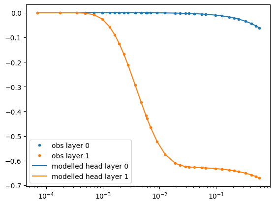
Calibrate parameters in multiple layers

Example showing how parameters can be optimized when multiple layers share the same parameter value.

ml = ttim.ModelMaq(
    kaq=[10.0, 10.0],
    z=(-10, -16, -18, -25),
    c=[10.0],
    Saq=[0.1, 1e-4],
    tmin=1e-5,
    tmax=1,
)
w = ttim.Well(ml, xw=0, yw=0, rw=0.1, tsandQ=[(0, 788)], layers=1)
ml.solve()
hobs0 = ml.head(robs, 0, tobs, layers=[0])[0]
hobs1 = ml.head(robs, 0, tobs, layers=[1])[0]

self.neq  1
solution complete

cal.parameters

	layers	optimal	std	perc_std	pmin	pmax	initial	inhoms	parray
kaq0_0_0	0	59.870508	0.660039	1.102444	-inf	inf	100.000	None	[[59.87050842164771]]
Saq0_0_0	0	0.000121	0.000004	3.590870	-inf	inf	0.001	None	[[0.00012119687595438834]]

cal = ttim.Calibrate(ml)
cal.set_parameter(
    name="kaq0_1", layers=[0, 1], initial=20.0, pmin=0.0, pmax=30.0
)  # layers 0 and 1 have the same k-value
cal.set_parameter(name="Saq0", layers=0, initial=1e-3, pmin=1e-5, pmax=0.2)
cal.set_parameter(name="Saq1", layers=1, initial=1e-3, pmin=1e-5, pmax=0.2)
cal.set_parameter(name="c1", layers=1, initial=1.0, pmin=0.1, pmax=200.0)
cal.series(name="obs0", x=robs, y=0, layer=0, t=tobs, h=hobs0)
cal.series(name="obs1", x=robs, y=0, layer=1, t=tobs, h=hobs1)
cal.fit(report=False)
display(cal.parameters)

...............
...
...
..
...
..............
...
....
.
...
..............
...
....
.
....
..............
..
....
.
....
...
Fit succeeded.

	layers	optimal	std	perc_std	pmin	pmax	initial	inhoms	parray
kaq0_1_0_1	[0, 1]	9.999129	2.442992e-04	0.002443	0.00000	30.0	20.000	None	[[9.999129279917383, 9.999129279917383]]
Saq0_0_0	0	0.100008	2.537887e-07	0.000254	0.00001	0.2	0.001	None	[[0.10000758667299027]]
Saq1_1_1	1	0.000100	8.769699e-10	0.000877	0.00001	0.2	0.001	None	[[9.999637318907012e-05]]
c1_1_1	1	9.999744	7.389049e-05	0.000739	0.10000	200.0	1.000	None	[[9.999743718534136]]

plt.semilogx(tobs, hobs0, ".C0", label="obs layer 0")
plt.semilogx(tobs, hobs1, ".C1", label="obs layer 1")

hm = ml.head(robs, 0, tobs)
plt.semilogx(tobs, hm[0], "C0", label="modelled head layer 0")
plt.semilogx(tobs, hm[1], "C1", label="modelled head layer 1")

plt.legend(loc="best");

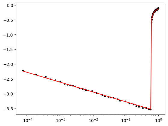
Generate data for head measured in well

tobs2 = np.hstack((tobs, np.arange(0.61, 1, 0.01)))

ml = ttim.ModelMaq(kaq=60, z=(-18, -25), Saq=1e-4, tmin=1e-5, tmax=1)
w = ttim.Well(ml, xw=0, yw=0, rw=0.3, res=0.02, tsandQ=[(0, 788), (0.6, 0)], layers=0)
ml.solve()
rnd = np.random.default_rng(2)
hobs2 = w.headinside(tobs2)[0] + 0.05 * rnd.random(len(tobs2))

self.neq  1
solution complete

cal = ttim.Calibrate(ml)
cal.set_parameter(name="kaq0", layers=0, initial=100)
cal.set_parameter(name="Saq0", layers=0, initial=1e-3)
cal.set_parameter_by_reference(name="res", parameter=w.res[:], initial=0.05)
cal.seriesinwell(name="obs1", element=w, t=tobs2, h=hobs2)
cal.fit()

..
...........................
...
.
...........................
...
.
............................
..
.
.............................
.
.
.............................
.
.
.............................
..
..............................
.
..............................
...............................
...............................
...............................
................................
...............................
Fit succeeded.

hm = w.headinside(tobs2)
plt.semilogx(tobs2, hobs2, ".k")
plt.semilogx(tobs2, hm[0], "r");