2. Slug Test - Falling Head#
This test is taken from examples of AQTESOLV.
Step 1. Import required libraries#
import matplotlib.pyplot as plt
import numpy as np
import pandas as pd

import ttim as ttm

plt.rcParams["figure.figsize"] = [5, 3]
Introduction and Conceptual Model#
In this notebook, we reproduce the work of Yang (2020) to check the TTim performance in analysing slug-test. We later compare the solution in TTim with the KGS analytical model (Hyder et al. 1994) implemented in AQTESOLV (Duffield, 2007).
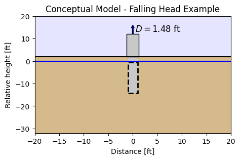
This slug test was reported in Batu (1998). A well partially penetrates a sandy unconfined aquifer that has a saturated depth of 32.57 ft. The top of the screen is located 0.47 ft below the water table and has 13.8 ft in length. The well and casing radii are 5 and 2 inches, respectively.
The slug displacement is 1.48 ft. Head change has been recorded at the slug well.
The conceptual model is seen in the figure below.
import matplotlib.pyplot as plt

##Now printing the conceptual model figure:

fig = plt.figure()
ax = fig.add_subplot(1, 1, 1)
# sky
sky = plt.Rectangle((-20, 2), width=50, height=20, fc="b", zorder=0, alpha=0.1)
ax.add_patch(sky)

# Aquifer:
ground = plt.Rectangle(
    (-20, -32.57),
    width=50,
    height=34.57,
    fc=np.array([209, 179, 127]) / 255,
    zorder=0,
    alpha=0.9,
)
ax.add_patch(ground)

well = plt.Rectangle(
    (-1, -(0.47 + 13.8)),
    width=2,
    height=(0.47 + 13.8) + 2,
    fc=np.array([200, 200, 200]) / 255,
    zorder=1,
)
ax.add_patch(well)

# Wellhead
wellhead = plt.Rectangle(
    (-1.25, 2),
    width=2.5,
    height=10,
    fc=np.array([200, 200, 200]) / 255,
    zorder=2,
    ec="k",
)
ax.add_patch(wellhead)

# Screen for the well:
screen = plt.Rectangle(
    (-1, -(0.47 + 13.8)),
    width=2,
    height=13.8,
    fc=np.array([200, 200, 200]) / 255,
    alpha=1,
    zorder=2,
    ec="k",
    ls="--",
)
screen.set_linewidth(2)
ax.add_patch(screen)
pumping_arrow = plt.Arrow(x=0, y=10, dx=0, dy=6, color="#00035b")
ax.add_patch(pumping_arrow)
ax.text(x=0.5, y=13, s=r"$ D = 1.48$ ft", fontsize="large")

# last line
line = plt.Line2D(xdata=[-200, 1200], ydata=[2, 2], color="k")
ax.add_line(line)

# water table
line = plt.Line2D(xdata=[-200, 1200], ydata=[0, 0], color="blue")
ax.add_line(line)


ax.set_xlim([-20, 20])
ax.set_ylim([-32, 20])
ax.set_xlabel("Distance [ft]")
ax.set_ylabel("Relative height [ft]")
ax.set_title("Conceptual Model - Falling Head Example");
Step 2. Set basic parameters#
Parameters here declared are already converted from feet and inches to meters
rw = 0.127  # well radius, m
rc = 0.0508  # well casing radius, m
L = 4.20624  # screen length, m
b = -9.9274  # aquifer thickness, m
zt = -0.1433  # depth to top of the screen, m
H0 = 0.4511  # initial displacement in the well, m
zb = zt - L  # bottom of the screen, m
Step 3. Converting slug displacement to volume#
Q = np.pi * rc**2 * H0
print(f"Slug: {Q:.5f} m^3")
Slug: 0.00366 m^3
Step 4. Load data#
Drawdown data is available in feet and seconds and are converted to meters and days
data = np.loadtxt("data/falling_head.txt", skiprows=2)
to = data[:, 0] / 60 / 60 / 24  # convert time from seconds to days
ho = (10 - data[:, 1]) * 0.3048  # convert drawdown from ft to meters
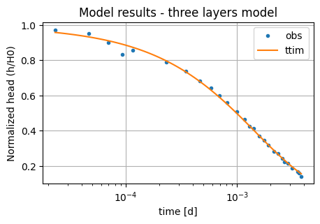
Step 5. Create First Model - three layers#
We begin with a model with just three layers. We arranged the layers to match the screen length. The first layer is located just above the screen, the second layer is located at the screen depths, and the last layer is just below the screen, up to the total aquifer depth.
We set the model in the same manner as in Slug 1 - Pratt County.
ml_0 = ttm.Model3D(kaq=10, z=[0, zt, zb, b], Saq=1e-4, tmin=1e-5, tmax=0.01)
w_0 = ttm.Well(ml_0, xw=0, yw=0, rw=rw, rc=rc, tsandQ=[(0, -Q)], layers=1, wbstype="slug")
ml_0.solve()
self.neq  1
solution complete
Step 6. Model calibration#
The procedures for calibration can be seen in Unconfined 1 - Vennebulten
We calibrate hydraulic conductivity and specific storage, as in the KGS model (Hyder et al. 1994).
ca_0 = ttm.Calibrate(ml_0)
ca_0.set_parameter(name="kaq0_2", initial=10)
ca_0.set_parameter(name="Saq0_2", initial=1e-4, pmin=1e-7)
ca_0.seriesinwell(name="obs", element=w_0, t=to, h=ho)
ca_0.fit(report=True)
.....................................
..............
Fit succeeded.
[[Fit Statistics]]
    # fitting method   = leastsq
    # function evals   = 48
    # data points      = 27
    # variables        = 2
    chi-square         = 0.00114579
    reduced chi-square = 4.5831e-05
    Akaike info crit   = -267.822514
    Bayesian info crit = -265.230840
[[Variables]]
    kaq0_2_0_2:  0.59961017 +/- 0.03384574 (5.64%) (init = 10)
    Saq0_2_0_2:  2.0941e-04 +/- 6.5493e-05 (31.28%) (init = 0.0001)
[[Correlations]] (unreported correlations are < 0.100)
    C(kaq0_2_0_2, Saq0_2_0_2) = -0.9720
/tmp/ipykernel_1336/3922385248.py:2: DeprecationWarning: Setting layers in the parameter name is deprecated. Set the layers= keyword argument for parameter 'kaq0_2' to silence this warning. The parameter name can still include layer info, but this will be ignored in a future version of TTim.
  ca_0.set_parameter(name="kaq0_2", initial=10)
/tmp/ipykernel_1336/3922385248.py:3: DeprecationWarning: Setting layers in the parameter name is deprecated. Set the layers= keyword argument for parameter 'Saq0_2' to silence this warning. The parameter name can still include layer info, but this will be ignored in a future version of TTim.
  ca_0.set_parameter(name="Saq0_2", initial=1e-4, pmin=1e-7)
display(ca_0.parameters)
print("RMSE:", ca_0.rmse())
| layers | optimal | std | perc_std | pmin | pmax | initial | inhoms | parray | |
|---|---|---|---|---|---|---|---|---|---|
| kaq0_2_0_2 | None | 0.599610 | 0.033846 | 5.644624 | -inf | inf | 10.0000 | None | [[0.5996101696554169, 0.5996101696554169, 0.59... |
| Saq0_2_0_2 | None | 0.000209 | 0.000065 | 31.275536 | 1.000000e-07 | inf | 0.0001 | None | [[0.00020940755465492789, 0.000209407554654927... |
RMSE: 0.006514334273111715
tm = np.logspace(np.log10(to[0]), np.log10(to[-1]), 100)
hm_0 = w_0.headinside(tm)
plt.semilogx(to, ho / H0, ".", label="obs")
plt.semilogx(tm, hm_0[0] / H0, label="ttim")
plt.xlabel("time [d]")
plt.ylabel("Normalized head (h/H0)")
plt.title("Model results - three layers model")
plt.legend()
plt.grid()
Step 7. Create Second Model - multi-layer model#
To investigate whether we can improve the model performance, we will create a multi-layer model. For this, we divide the previous second and third layers into 0.5 m thick layers:
# Determine elevation of each layer.
# Thickness of each layer is set to be 0.5 m.
z0 = np.arange(zt, zb, -0.5)
z1 = np.arange(zb, b, -0.5)
zlay = np.append(z0, z1)
zlay = np.append(zlay, b)
zlay = np.insert(zlay, 0, 0)
nlay = len(zlay) - 1  # number of layers
Saq_1 = 1e-4 * np.ones(nlay)
Saq_1[0] = 0.1
ml_1 = ttm.Model3D(
    kaq=10, z=zlay, Saq=Saq_1, kzoverkh=1, tmin=1e-5, tmax=0.01, phreatictop=True
)
w_1 = ttm.Well(
    ml_1,
    xw=0,
    yw=0,
    rw=rw,
    tsandQ=[(0, -Q)],
    layers=[1, 2, 3, 4, 5, 6, 7, 8],
    rc=rc,
    wbstype="slug",
)
ml_1.solve()
self.neq  8
solution complete
Step 8. Calibration of multi-layer model#
ca_1 = ttm.Calibrate(ml_1)
ca_1.set_parameter(name="kaq0_21", initial=10, pmin=0)
ca_1.set_parameter(name="Saq0_21", initial=1e-4, pmin=0)
ca_1.seriesinwell(name="obs", element=w_1, t=to, h=ho)
ca_1.fit(report=True)
.
.........
.
.........
.
.........
.
.
Fit succeeded.
[[Fit Statistics]]
    # fitting method   = leastsq
    # function evals   = 29
    # data points      = 27
    # variables        = 2
    chi-square         = 0.00108525
    reduced chi-square = 4.3410e-05
    Akaike info crit   = -269.288034
    Bayesian info crit = -266.696360
[[Variables]]
    kaq0_21_0_21:  0.49534075 +/- 0.02256321 (4.56%) (init = 10)
    Saq0_21_0_21:  4.0606e-04 +/- 1.0394e-04 (25.60%) (init = 0.0001)
[[Correlations]] (unreported correlations are < 0.100)
    C(kaq0_21_0_21, Saq0_21_0_21) = -0.9593
/tmp/ipykernel_1336/159376845.py:2: DeprecationWarning: Setting layers in the parameter name is deprecated. Set the layers= keyword argument for parameter 'kaq0_21' to silence this warning. The parameter name can still include layer info, but this will be ignored in a future version of TTim.
  ca_1.set_parameter(name="kaq0_21", initial=10, pmin=0)
/tmp/ipykernel_1336/159376845.py:3: DeprecationWarning: Setting layers in the parameter name is deprecated. Set the layers= keyword argument for parameter 'Saq0_21' to silence this warning. The parameter name can still include layer info, but this will be ignored in a future version of TTim.
  ca_1.set_parameter(name="Saq0_21", initial=1e-4, pmin=0)
display(ca_1.parameters)
print("RMSE:", ca_1.rmse())
| layers | optimal | std | perc_std | pmin | pmax | initial | inhoms | parray | |
|---|---|---|---|---|---|---|---|---|---|
| kaq0_21_0_21 | None | 0.495341 | 0.022563 | 4.555088 | 0.0 | inf | 10.0000 | None | [[0.49534074554701535, 0.49534074554701535, 0.... |
| Saq0_21_0_21 | None | 0.000406 | 0.000104 | 25.597292 | 0.0 | inf | 0.0001 | None | [[0.0004060577460704984, 0.0004060577460704984... |
RMSE: 0.0063399175663631895
RMSE has just slightly improved, and the parameter values are more or less similar to the previous values. However, AIC has improved significantly.
Step 10. Analysis and comparison of simulated values#
We now compare the values in TTim and add the results of the AQTESOLV modelling reported by Yang (2020).
ta = pd.DataFrame(
    columns=["k [m/d]", "Ss [1/m]"],
    index=["AQTESOLV", "ttim-three", "ttim-multi"],
)
ta.loc["ttim-three"] = ca_0.parameters["optimal"].values
ta.loc["ttim-multi"] = ca_1.parameters["optimal"].values
ta.loc["AQTESOLV"] = [2.616, 7.894e-5]
ta["RMSE"] = [
    0.001197,
    round(ca_0.rmse(), 6),
    round(ca_1.rmse(), 6),
]
ta.style.set_caption("Comparison of parameter values and error under different models")
| k [m/d] | Ss [1/m] | RMSE | |
|---|---|---|---|
| AQTESOLV | 2.616000 | 0.000079 | 0.001197 |
| ttim-three | 0.599610 | 0.000209 | 0.006514 |
| ttim-multi | 0.495341 | 0.000406 | 0.006340 |
AQTESOLV parameters are quite different from the set parameters in TTim. It also has a better RMSE performance. All TTim models are very similar to each other. However, the multi-layer models performed better.
References#
Batu, V., 1998. Aquifer hydraulics: a comprehensive guide to hydrogeologic data analysis. John Wiley & Sons
Hyder, Z., Butler Jr, J.J., McElwee, C.D., Liu, W., 1994. Slug tests in partially penetrating wells. Water Resources Research 30, 2945–2957.
Duffield, G.M., 2007. AQTESOLV for Windows Version 4.5 User’s Guide, HydroSOLVE, Inc., Reston, VA.
Yang, Xinzhu (2020) Application and comparison of different methodsfor aquifer test analysis using TTim. Master Thesis, Delft University of Technology (TUDelft), Delft, The Netherlands.