1. Leaky Aquifer Test - Dalem Example#

This example is taken from Kruseman et al. (1970)

Import packages#

import matplotlib.pyplot as plt
import numpy as np
import pandas as pd

import ttim as ttm

plt.rcParams["figure.figsize"] = [5, 3]

Introduction and Conceptual Model#

In many situations, we cannot ignore the leakage potential of overlying and underlying formations to aquifers, and we cannot conceptualize them as confined. TTim is capable of modelling and adjusting parameters to leaky, semi-confined aquifers.

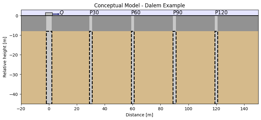
The current is the pumping test from Dalem (Kruseman et al., 1970), the Netherlands. The hydrogeological cross-section is composed of the following elements: an initial 8 m deep aquitard layer, followed by an aquifer from 8 m to 45 m depth. The layer underlying the aquifer is considered an aquiclude. The pumping well is placed at the aquifer, and drawdown is recorded at four different piezometers, 30, 60, 90 and 120 m away from the well. The pumping lasted 8 hours in total at a rate of 761 m\(^3\)/d. There is a river 1500 m away from the well. The tide affects both river and well levels. Data has been previously corrected for the tide effect.

In this benchmarking exercise, we will simulate two different conceptual models. The first model assumes no storage in the aquitard. That matches most analytical solutions for leaky-aquitard (Kruseman et al., 1970). In the second model, we will explore TTim’s flexibility for modelling and add storage as an additional parameter to be adjusted. Finally, we compare the results of the models with other software.

The figures below resume the conceptual models:

Show code cell source

Hide code cell source

# Conceptual Model 1
import matplotlib.pyplot as plt

##Now printing the conceptual model figure:

fig = plt.figure(figsize=(10, 4))
ax = fig.add_subplot(1, 1, 1)
# sky
sky = plt.Rectangle((-20, 0), width=170, height=3, fc="b", zorder=0, alpha=0.1)
ax.add_patch(sky)

# Aquifer:
ground = plt.Rectangle(
    (-20, -45),
    width=170,
    height=37,
    fc=np.array([209, 179, 127]) / 255,
    zorder=0,
    alpha=0.9,
)
ax.add_patch(ground)

# Confining bed:
confining_unit = plt.Rectangle(
    (-20, -8),
    width=170,
    height=8,
    fc=np.array([100, 100, 100]) / 255,
    zorder=0,
    alpha=0.7,
)
ax.add_patch(confining_unit)

well = plt.Rectangle(
    (-2, -45), width=4, height=45, fc=np.array([200, 200, 200]) / 255, zorder=1
)
ax.add_patch(well)

# Wellhead
wellhead = plt.Rectangle(
    (-2.5, 0), width=5, height=1.5, fc=np.array([200, 200, 200]) / 255, zorder=2, ec="k"
)
ax.add_patch(wellhead)

# Screen for the well:
screen = plt.Rectangle(
    (-2, -45),
    width=4,
    height=37,
    fc=np.array([200, 200, 200]) / 255,
    alpha=1,
    zorder=2,
    ec="k",
    ls="--",
)
screen.set_linewidth(2)
ax.add_patch(screen)
pumping_arrow = plt.Arrow(x=2.5, y=0.75, dx=5, dy=0, color="#00035b")
ax.add_patch(pumping_arrow)
ax.text(x=7.5, y=0.75, s=r"$ Q$", fontsize="large")
# Piezometers
piez1 = plt.Rectangle(
    (29, -45), width=2, height=45, fc=np.array([200, 200, 200]) / 255, zorder=1
)
screen_piez_1 = plt.Rectangle(
    (29, -45),
    width=2,
    height=37,
    fc=np.array([200, 200, 200]) / 255,
    alpha=1,
    zorder=2,
    ec="k",
    ls="--",
)
screen_piez_1.set_linewidth(2)

piez2 = plt.Rectangle(
    (59, -45), width=2, height=45, fc=np.array([200, 200, 200]) / 255, zorder=1
)
screen_piez_2 = plt.Rectangle(
    (59, -45),
    width=2,
    height=37,
    fc=np.array([200, 200, 200]) / 255,
    alpha=1,
    zorder=2,
    ec="k",
    ls="--",
)
screen_piez_2.set_linewidth(2)

piez3 = plt.Rectangle(
    (89, -45), width=2, height=45, fc=np.array([200, 200, 200]) / 255, zorder=1
)
screen_piez_3 = plt.Rectangle(
    (89, -45),
    width=2,
    height=37,
    fc=np.array([200, 200, 200]) / 255,
    alpha=1,
    zorder=2,
    ec="k",
    ls="--",
)
screen_piez_3.set_linewidth(2)

piez4 = plt.Rectangle(
    (119, -45), width=2, height=45, fc=np.array([200, 200, 200]) / 255, zorder=1
)
screen_piez_4 = plt.Rectangle(
    (119, -45),
    width=2,
    height=37,
    fc=np.array([200, 200, 200]) / 255,
    alpha=1,
    zorder=2,
    ec="k",
    ls="--",
)
screen_piez_4.set_linewidth(2)

ax.add_patch(piez1)
ax.add_patch(screen_piez_1)
ax.add_patch(piez2)
ax.add_patch(screen_piez_2)
ax.add_patch(piez3)
ax.add_patch(screen_piez_3)
ax.add_patch(piez4)
ax.add_patch(screen_piez_4)

# last line
line = plt.Line2D(xdata=[-200, 1200], ydata=[0, 0], color="k")
ax.add_line(line)

ax.text(x=29, y=0.75, s="P30", fontsize="large")
ax.text(x=59, y=0.75, s="P60", fontsize="large")
ax.text(x=89, y=0.75, s="P90", fontsize="large")
ax.text(x=119, y=0.75, s="P120", fontsize="large")


ax.set_xlim([-20, 150])
ax.set_ylim([-45, 3])
ax.set_xlabel("Distance [m]")
ax.set_ylabel("Relative height [m]")
ax.set_title("Conceptual Model - Dalem Example");

../_images/5ed596d051b0d9ffd5f0572f018b776b781e5167ca31a716d1b9422c76ee6c32.png

Set basic parameters#

H = 37  # aquifer thickness, m
zt = -8  # top boundary of aquifer, m
zb = zt - H  # bottom boundary of the aquifer, m
Q = 761  # constant pumping rate, m^3/d
t = 0.34  # total pumping time, d

Create conceptual model#

Until so far, we have only considered impermeable upper boundaries in our model. This assumption, however, is not sufficient in many situations where there is enough leakage from above to influence flow results. TTim can simulate such semi-confined conditions in ModelMaq setup with the parameter: topboundary = 'semi'.

When we do this, ModelMaq assumes a leaky layer is on top of the uppermost aquifer. A leaky layer in TTim only has vertical flow and is characterized by the parameters resistance to vertical flow (c) and storage (Sll). The specific flux is computed as (Bakker, 2013):

\[q_n = \frac{h_n-h_{n-1}}{c_n}\]

where \(q_n\) is the vertical flux from layer \(n\) to layer \(n-1\), \(h_n\) is the head in layer \(n\) and \(c_n\) is the vertical resistance to flow. \(c_n\) is computed as: \(H_n/k_n\) where, \(H_n\) is the leaky-layer thickness and \(k_n\) the vertical hydraulic conductance. \(c_n\) is the inverse of the parameter Leakance (\(L_n = 1/c_n\)), that is used in MODFLOW (Harbaugh, 2005) or analytical solutions of leaky-layers, such as in Hantush (1955).

Specifying topboundary = 'semi' means that we also have to set the parameters for the aquitard overlying the aquifer formation. Thus, even though we have only one aquifer, we have to set an additional element to the z array, which is the top of the aquitard formation:

z = [0,zt,zb]: 0 is the depth of the aquitard overlying the aquifer, zt and zb are the top and bottom of the aquifer

In this first example, we also have to set the resistance of the aquitard:

c = 500: We will calibrate this value later.

For now, we are ignoring the storage of this leaky layer. In this case, TTim will consider the head remains fixed above the leaky layer.

More explanations over how TTim sets up the ModelMaq model can be seen in the notebooks:

# unkonwn parameters: kaq, Saq, c
ml = ttm.ModelMaq(
    kaq=10, z=[0, zt, zb], c=500, Saq=0.001, topboundary="semi", tmin=0.01, tmax=1
)
w = ttm.Well(ml, xw=0, yw=0, tsandQ=[(0, Q), (0.34, 0)])
ml.solve(silent="True")

Load data of four observation wells.#

The data for each observation well is organized in text files where the first column is the time data in days and the second is the drawdown in meters, corrected for the tide effect. Here we are also declaring the distance from the pumping well:

# data of observation well 30 m away from pumping well
data1 = np.loadtxt("data/dalem_p30.txt", skiprows=1)
t1 = data1[:, 0]
h1 = data1[:, 1]
r1 = 30
# data of observation well 60 m away from pumping well
data2 = np.loadtxt("data/dalem_p60.txt", skiprows=1)
t2 = data2[:, 0]
h2 = data2[:, 1]
r2 = 60
# data of observation well 90 m away from pumping well
data3 = np.loadtxt("data/dalem_p90.txt", skiprows=1)
t3 = data3[:, 0]
h3 = data3[:, 1]
r3 = 90
# data of observation well 120 m away from pumping well
data4 = np.loadtxt("data/dalem_p120.txt", skiprows=1)
t4 = data4[:, 0]
h4 = data4[:, 1]
r4 = 120

Step 5. Model Calibration#

Step 5.1. Calibration with three datasets (excluding one piezometer at a time)#

We begin investigating the model calibration if we exclude one piezometer at a time. Hence, we look into the influence of each piezometer on parameter calibration.

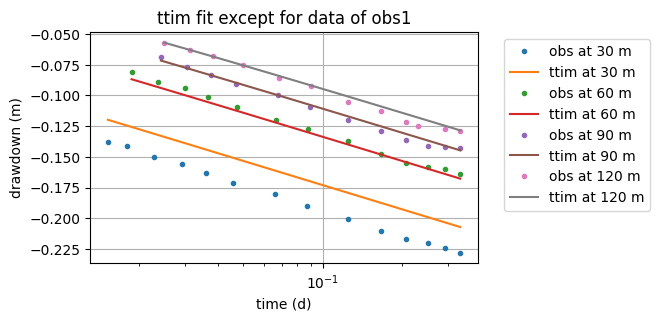
5.1.1. Calibration without obs1#

ca1 = ttm.Calibrate(ml)
ca1.set_parameter(name="kaq0", initial=10, pmin=1, pmax=100)
ca1.set_parameter(name="Saq0", initial=1e-4, pmin=1e-5, pmax=1e-3)
ca1.set_parameter(name="c0", initial=100, pmin=20, pmax=1e5)
ca1.series(name="obs2", x=r2, y=0, layer=0, t=t2, h=h2)
ca1.series(name="obs3", x=r3, y=0, layer=0, t=t3, h=h3)
ca1.series(name="obs4", x=r4, y=0, layer=0, t=t4, h=h4)
ca1.fit()
ca1.parameters.loc[:, ["optimal"]]

..........................................................
Fit succeeded.

/tmp/ipykernel_1247/2416328086.py:2: DeprecationWarning: Setting layers in the parameter name is deprecated. Set the layers= keyword argument for parameter 'kaq0' to silence this warning. The parameter name can still include layer info, but this will be ignored in a future version of TTim.
  ca1.set_parameter(name="kaq0", initial=10, pmin=1, pmax=100)
/tmp/ipykernel_1247/2416328086.py:3: DeprecationWarning: Setting layers in the parameter name is deprecated. Set the layers= keyword argument for parameter 'Saq0' to silence this warning. The parameter name can still include layer info, but this will be ignored in a future version of TTim.
  ca1.set_parameter(name="Saq0", initial=1e-4, pmin=1e-5, pmax=1e-3)
/tmp/ipykernel_1247/2416328086.py:4: DeprecationWarning: Setting layers in the parameter name is deprecated. Set the layers= keyword argument for parameter 'c0' to silence this warning. The parameter name can still include layer info, but this will be ignored in a future version of TTim.
  ca1.set_parameter(name="c0", initial=100, pmin=20, pmax=1e5)

	optimal
kaq0_0_0	57.518329
Saq0_0_0	0.000033
c0_0_0	99999.874905

print("rmse:", ca1.rmse())
ha1 = ml.head(r1, 0, t1)
plt.semilogx(t1, h1, ".", label="obs at 30 m")
plt.semilogx(t1, ha1[0], label="ttim at 30 m")
ha2 = ml.head(r2, 0, t2)
plt.semilogx(t2, h2, ".", label="obs at 60 m")
plt.semilogx(t2, ha2[0], label="ttim at 60 m")
ha3 = ml.head(r3, 0, t3)
plt.semilogx(t3, h3, ".", label="obs at 90 m")
plt.semilogx(t3, ha3[0], label="ttim at 90 m")
ha4 = ml.head(r4, 0, t4)
plt.semilogx(t4, h4, ".", label="obs at 120 m")
plt.semilogx(t4, ha4[0], label="ttim at 120 m")
plt.xlabel("time (d)")
plt.ylabel("drawdown (m)")
plt.title("ttim fit except for data of obs1")
plt.legend(bbox_to_anchor=(1.05, 1))
plt.grid()

rmse: 0.0032364785374164244

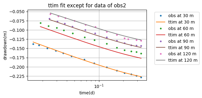
../_images/6b9049bc1808b194abbccf658d87b791ed7ad7f52264a82cf3cec0c5b5185d65.png

5.1.2. Calibration without obs2#

ca2 = ttm.Calibrate(ml)
ca2.set_parameter(name="kaq0", initial=10, pmin=1, pmax=100)
ca2.set_parameter(name="Saq0", initial=1e-4, pmin=1e-5, pmax=1e-3)
ca2.set_parameter(name="c0", initial=1000, pmin=100, pmax=1e6)
ca2.series(name="obs1", x=r1, y=0, layer=0, t=t1, h=h1)
ca2.series(name="obs3", x=r3, y=0, layer=0, t=t3, h=h3)
ca2.series(name="obs4", x=r4, y=0, layer=0, t=t4, h=h4)
ca2.fit()
ca2.parameters.loc[:, ["optimal"]]

......
......
.....................................................
Fit succeeded.

/tmp/ipykernel_1247/1775893712.py:2: DeprecationWarning: Setting layers in the parameter name is deprecated. Set the layers= keyword argument for parameter 'kaq0' to silence this warning. The parameter name can still include layer info, but this will be ignored in a future version of TTim.
  ca2.set_parameter(name="kaq0", initial=10, pmin=1, pmax=100)
/tmp/ipykernel_1247/1775893712.py:3: DeprecationWarning: Setting layers in the parameter name is deprecated. Set the layers= keyword argument for parameter 'Saq0' to silence this warning. The parameter name can still include layer info, but this will be ignored in a future version of TTim.
  ca2.set_parameter(name="Saq0", initial=1e-4, pmin=1e-5, pmax=1e-3)
/tmp/ipykernel_1247/1775893712.py:4: DeprecationWarning: Setting layers in the parameter name is deprecated. Set the layers= keyword argument for parameter 'c0' to silence this warning. The parameter name can still include layer info, but this will be ignored in a future version of TTim.
  ca2.set_parameter(name="c0", initial=1000, pmin=100, pmax=1e6)

	optimal
kaq0_0_0	45.026452
Saq0_0_0	0.000044
c0_0_0	349.139321

print("rmse:", ca2.rmse())
hb1 = ml.head(r1, 0, t1)
plt.semilogx(t1, h1, ".", label="obs at 30 m")
plt.semilogx(t1, hb1[0], label="ttim at 30 m")
hb2 = ml.head(r2, 0, t2)
plt.semilogx(t2, h2, ".", label="obs at 60 m")
plt.semilogx(t2, hb2[0], label="ttim at 60 m")
hb3 = ml.head(r3, 0, t3)
plt.semilogx(t3, h3, ".", label="obs at 90 m")
plt.semilogx(t3, hb3[0], label="ttim at 90 m")
hb4 = ml.head(r4, 0, t4)
plt.semilogx(t4, h4, ".", label="obs at 120 m")
plt.semilogx(t4, hb4[0], label="ttim at 120 m")
plt.xlabel("time(d)")
plt.ylabel("drawdown(m)")
plt.title("ttim fit except for data of obs2")
plt.legend(bbox_to_anchor=(1.05, 1))
plt.grid()

rmse: 0.0026334102194292175

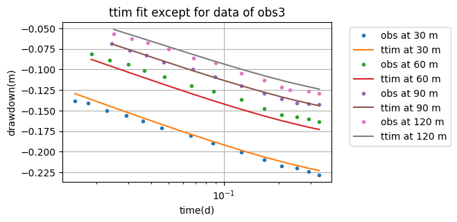
../_images/d1e0523b1556e3c74a9e4f9d582c0b1bdb30fed69c99da31e4e160d5b1a00ed9.png

5.1.3. Calibration without obs3#

ca3 = ttm.Calibrate(ml)
ca3.set_parameter(name="kaq0", initial=10, pmin=1, pmax=100)
ca3.set_parameter(name="Saq0", initial=1e-4, pmin=1e-5, pmax=1e-3)
ca3.set_parameter(name="c0", initial=1000, pmin=100, pmax=1e6)
ca3.series(name="obs1", x=r1, y=0, layer=0, t=t1, h=h1)
ca3.series(name="obs3", x=r2, y=0, layer=0, t=t2, h=h2)
ca3.series(name="obs4", x=r4, y=0, layer=0, t=t4, h=h4)
ca3.fit()
ca3.parameters.loc[:, ["optimal"]]

..........
........
....................................
Fit succeeded.

/tmp/ipykernel_1247/3668376910.py:2: DeprecationWarning: Setting layers in the parameter name is deprecated. Set the layers= keyword argument for parameter 'kaq0' to silence this warning. The parameter name can still include layer info, but this will be ignored in a future version of TTim.
  ca3.set_parameter(name="kaq0", initial=10, pmin=1, pmax=100)
/tmp/ipykernel_1247/3668376910.py:3: DeprecationWarning: Setting layers in the parameter name is deprecated. Set the layers= keyword argument for parameter 'Saq0' to silence this warning. The parameter name can still include layer info, but this will be ignored in a future version of TTim.
  ca3.set_parameter(name="Saq0", initial=1e-4, pmin=1e-5, pmax=1e-3)
/tmp/ipykernel_1247/3668376910.py:4: DeprecationWarning: Setting layers in the parameter name is deprecated. Set the layers= keyword argument for parameter 'c0' to silence this warning. The parameter name can still include layer info, but this will be ignored in a future version of TTim.
  ca3.set_parameter(name="c0", initial=1000, pmin=100, pmax=1e6)

	optimal
kaq0_0_0	45.204890
Saq0_0_0	0.000048
c0_0_0	318.723651

print("rmse:", ca3.rmse())
hc1 = ml.head(r1, 0, t1)
plt.semilogx(t1, h1, ".", label="obs at 30 m")
plt.semilogx(t1, hc1[0], label="ttim at 30 m")
hc2 = ml.head(r2, 0, t2)
plt.semilogx(t2, h2, ".", label="obs at 60 m")
plt.semilogx(t2, hc2[0], label="ttim at 60 m")
hc3 = ml.head(r3, 0, t3)
plt.semilogx(t3, h3, ".", label="obs at 90 m")
plt.semilogx(t3, hc3[0], label="ttim at 90 m")
hc4 = ml.head(r4, 0, t4)
plt.semilogx(t4, h4, ".", label="obs at 120 m")
plt.semilogx(t4, hc4[0], label="ttim at 120 m")
plt.xlabel("time(d)")
plt.ylabel("drawdown(m)")
plt.title("ttim fit except for data of obs3")
plt.legend(bbox_to_anchor=(1.05, 1))
plt.grid()

rmse: 0.00672584585950414

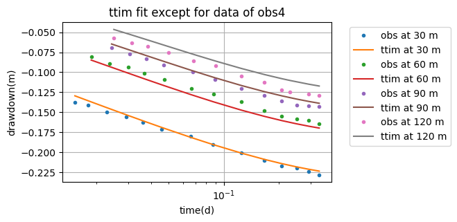
../_images/568d844c65a633b715a1346462e5ead038a3a347bfff9bbc1134035624c0583b.png

5.1.4. Calibration without obs4#

ca4 = ttm.Calibrate(ml)
ca4.set_parameter(name="kaq0", initial=10, pmin=1, pmax=100)
ca4.set_parameter(name="Saq0", initial=1e-4, pmin=1e-5, pmax=1e-3)
ca4.set_parameter(name="c0", initial=1000, pmin=100, pmax=1e6)
ca4.series(name="obs1", x=r1, y=0, layer=0, t=t1, h=h1)
ca4.series(name="obs3", x=r2, y=0, layer=0, t=t2, h=h2)
ca4.series(name="obs4", x=r3, y=0, layer=0, t=t3, h=h3)
ca4.fit()
ca4.parameters.loc[:, ["optimal"]]

.................................
Fit succeeded.

/tmp/ipykernel_1247/2845238728.py:2: DeprecationWarning: Setting layers in the parameter name is deprecated. Set the layers= keyword argument for parameter 'kaq0' to silence this warning. The parameter name can still include layer info, but this will be ignored in a future version of TTim.
  ca4.set_parameter(name="kaq0", initial=10, pmin=1, pmax=100)
/tmp/ipykernel_1247/2845238728.py:3: DeprecationWarning: Setting layers in the parameter name is deprecated. Set the layers= keyword argument for parameter 'Saq0' to silence this warning. The parameter name can still include layer info, but this will be ignored in a future version of TTim.
  ca4.set_parameter(name="Saq0", initial=1e-4, pmin=1e-5, pmax=1e-3)
/tmp/ipykernel_1247/2845238728.py:4: DeprecationWarning: Setting layers in the parameter name is deprecated. Set the layers= keyword argument for parameter 'c0' to silence this warning. The parameter name can still include layer info, but this will be ignored in a future version of TTim.
  ca4.set_parameter(name="c0", initial=1000, pmin=100, pmax=1e6)

	optimal
kaq0_0_0	41.720987
Saq0_0_0	0.000058
c0_0_0	180.966613

print("rmse:", ca4.rmse())
hd1 = ml.head(r1, 0, t1)
plt.semilogx(t1, h1, ".", label="obs at 30 m")
plt.semilogx(t1, hd1[0], label="ttim at 30 m")
hd2 = ml.head(r2, 0, t2)
plt.semilogx(t2, h2, ".", label="obs at 60 m")
plt.semilogx(t2, hd2[0], label="ttim at 60 m")
hd3 = ml.head(r3, 0, t3)
plt.semilogx(t3, h3, ".", label="obs at 90 m")
plt.semilogx(t3, hd3[0], label="ttim at 90 m")
hd4 = ml.head(r4, 0, t4)
plt.semilogx(t4, h4, ".", label="obs at 120 m")
plt.semilogx(t4, hd4[0], label="ttim at 120 m")
plt.xlabel("time(d)")
plt.ylabel("drawdown(m)")
plt.title("ttim fit except for data of obs4")
plt.legend(bbox_to_anchor=(1.05, 1))
plt.grid()

rmse: 0.005405897674203384

../_images/534c710556918090e5e3e68b99209c0bf40ebce1fa6e2252ddcc0ba1e51ae028.png

5.1.4. Summary of results of the simulations missing one observation#

t = pd.DataFrame(
    columns=["k [m/d]", "Ss [1/m]", "c [d]"],
    index=[
        "Data at 30 m removed",
        "Data at 60 m removed",
        "Data at 90 m removed",
        "Data at 120 m removed",
    ],
)
t.loc["Data at 30 m removed"] = ca1.parameters["optimal"].values
t.loc["Data at 60 m removed"] = ca2.parameters["optimal"].values
t.loc["Data at 90 m removed"] = ca3.parameters["optimal"].values
t.loc["Data at 120 m removed"] = ca4.parameters["optimal"].values
rmse = [ca1.rmse(), ca2.rmse(), ca3.rmse(), ca4.rmse()]
t["RMSE"] = rmse
t

	k [m/d]	Ss [1/m]	c [d]	RMSE
Data at 30 m removed	57.518329	0.000033	99999.874905	0.003236
Data at 60 m removed	45.026452	0.000044	349.139321	0.002633
Data at 90 m removed	45.20489	0.000048	318.723651	0.006726
Data at 120 m removed	41.720987	0.000058	180.966613	0.005406

The values for hydraulic conductivity and specific storage changed slightly for every simulation. However, the resistance of the aquitard layer varied significantly, indicating that this parameter is not uniform in the region investigated.

Step 5.2. Calibrate with four datasets simultaneously:#

Now we calibrate the same model but with all four observation wells considered.

# unkonwn parameters: kaq, Saq, c
m_1 = ttm.ModelMaq(
    kaq=10, z=[0, zt, zb], c=500, Saq=0.001, topboundary="semi", tmin=0.01, tmax=1
)
w_1 = ttm.Well(m_1, xw=0, yw=0, tsandQ=[(0, Q), (0.34, 0)])
m_1.solve(silent="True")

c0 = ttm.Calibrate(ml)
c0.set_parameter(name="kaq0", initial=10)
c0.set_parameter(name="Saq0", initial=1e-4)
c0.set_parameter(name="c0", initial=500, pmin=0)
c0.series(name="obs1", x=30, y=0, t=t1, h=h1, layer=0)
c0.series(name="obs2", x=60, y=0, t=t2, h=h2, layer=0)
c0.series(name="obs3", x=90, y=0, t=t3, h=h3, layer=0)
c0.series(name="obs4", x=120, y=0, t=t4, h=h4, layer=0)
c0.fit()
c0.parameters.loc[:, ["optimal"]]

..
...
.....................................
Fit succeeded.

/tmp/ipykernel_1247/834188826.py:2: DeprecationWarning: Setting layers in the parameter name is deprecated. Set the layers= keyword argument for parameter 'kaq0' to silence this warning. The parameter name can still include layer info, but this will be ignored in a future version of TTim.
  c0.set_parameter(name="kaq0", initial=10)
/tmp/ipykernel_1247/834188826.py:3: DeprecationWarning: Setting layers in the parameter name is deprecated. Set the layers= keyword argument for parameter 'Saq0' to silence this warning. The parameter name can still include layer info, but this will be ignored in a future version of TTim.
  c0.set_parameter(name="Saq0", initial=1e-4)
/tmp/ipykernel_1247/834188826.py:4: DeprecationWarning: Setting layers in the parameter name is deprecated. Set the layers= keyword argument for parameter 'c0' to silence this warning. The parameter name can still include layer info, but this will be ignored in a future version of TTim.
  c0.set_parameter(name="c0", initial=500, pmin=0)

	optimal
kaq0_0_0	45.332095
Saq0_0_0	0.000048
c0_0_0	331.179789

hm_11 = ml.head(r1, 0, t1)
hm_12 = ml.head(r2, 0, t2)
hm_13 = ml.head(r3, 0, t3)
hm_14 = ml.head(r4, 0, t4)
print("rmse:", c0.rmse())
plt.semilogx(t1, h1, ".", label="obs at 30 m")
plt.semilogx(t1, hm_11[0], label="ttim at 30 m")
plt.semilogx(t2, h2, ".", label="obs at 60 m")
plt.semilogx(t2, hm_12[0], label="ttim at 60 m")
plt.semilogx(t3, h3, ".", label="obs at 90 m")
plt.semilogx(t3, hm_13[0], label="ttim at 90 m")
plt.semilogx(t4, h4, ".", label="obs at 120 m")
plt.semilogx(t4, hm_14[0], label="ttim at 120 m")
plt.xlabel("time(d)")
plt.ylabel("drawdown(m)")
plt.title("model with leakage only")
plt.legend(bbox_to_anchor=(1.05, 1))
plt.grid()

rmse: 0.005916842041771006

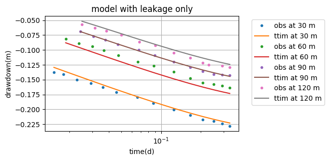
../_images/18d6d2d96f4996b697b79a534c9951215efac12147be3ce096b73e3d74d5a12c.png

The overall fit is relatively good. Comparing the new model to the three previous models, the adjusted parameters seem to be in between the previously computed values.

Step 6. Alternative Model Aquitard with leakage & storage#

The second conceptualization for the Dalem test is to consider the storage in the aquitard. Hence, we define the Sll parameter in the model building class ModelMaq:

# unkonwn parameters: kaq, Saq, c, Sll
m_2 = ttm.ModelMaq(
    kaq=10,
    z=[0, zt, zb],
    c=500,
    Saq=0.001,
    Sll=0.001,
    topboundary="semi",
    tmin=0.01,
    tmax=1,
)
w_2 = ttm.Well(m_2, xw=0, yw=0, tsandQ=[(0, Q), (0.34, 0)])
m_2.solve(silent="True")

Step 7. Calibration of Alternative Model#

We follow the same previous steps for calibration, but now we add the additional Sll parameter.

## Check why the errors in the pmin of the Sll adjustment
c1 = ttm.Calibrate(m_2)
c1.set_parameter(name="kaq0", initial=10)
c1.set_parameter(name="Saq0", initial=1e-4, pmin=0)
c1.set_parameter(name="c0", initial=500, pmin=0, pmax=1000)
c1.set_parameter(name="Sll0", initial=1e-6, pmin=1e-12, pmax=0.01)
c1.series(name="obs1", x=30, y=0, t=t1, h=h1, layer=0)
c1.series(name="obs2", x=60, y=0, t=t2, h=h2, layer=0)
c1.series(name="obs3", x=90, y=0, t=t3, h=h3, layer=0)
c1.series(name="obs4", x=120, y=0, t=t4, h=h4, layer=0)
c1.fit()
c1.parameters.loc[:, ["optimal"]]

.......
........
...................................................
.......
........
.....................................................
......
........
....................................................
.......
.......
.....................................................
......
........
.....................................................
......
........
.....................................................
.....
.........
.....................................................
.....
.........
.....................................................
.....
.........
....................................................
......
........
......................................................
.....
........
......................................................
.....
.
Fit succeeded.

/tmp/ipykernel_1247/3931242810.py:3: DeprecationWarning: Setting layers in the parameter name is deprecated. Set the layers= keyword argument for parameter 'kaq0' to silence this warning. The parameter name can still include layer info, but this will be ignored in a future version of TTim.
  c1.set_parameter(name="kaq0", initial=10)
/tmp/ipykernel_1247/3931242810.py:4: DeprecationWarning: Setting layers in the parameter name is deprecated. Set the layers= keyword argument for parameter 'Saq0' to silence this warning. The parameter name can still include layer info, but this will be ignored in a future version of TTim.
  c1.set_parameter(name="Saq0", initial=1e-4, pmin=0)
/tmp/ipykernel_1247/3931242810.py:5: DeprecationWarning: Setting layers in the parameter name is deprecated. Set the layers= keyword argument for parameter 'c0' to silence this warning. The parameter name can still include layer info, but this will be ignored in a future version of TTim.
  c1.set_parameter(name="c0", initial=500, pmin=0, pmax=1000)
/tmp/ipykernel_1247/3931242810.py:6: DeprecationWarning: Setting layers in the parameter name is deprecated. Set the layers= keyword argument for parameter 'Sll0' to silence this warning. The parameter name can still include layer info, but this will be ignored in a future version of TTim.
  c1.set_parameter(name="Sll0", initial=1e-6, pmin=1e-12, pmax=0.01)

	optimal
kaq0_0_0	44.398308
Saq0_0_0	0.000040
c0_0_0	885.737117
Sll0_0_0	0.000531

hm_21 = m_2.head(r1, 0, t1)
hm_22 = m_2.head(r2, 0, t2)
hm_23 = m_2.head(r3, 0, t3)
hm_24 = m_2.head(r4, 0, t4)
print("rmse:", c1.rmse())
plt.semilogx(t1, h1, ".", label="obs at 30 m")
plt.semilogx(t1, hm_21[0], label="ttim at 30 m")
plt.semilogx(t2, h2, ".", label="obs at 60 m")
plt.semilogx(t2, hm_22[0], label="ttim at 60 m")
plt.semilogx(t3, h3, ".", label="obs at 90 m")
plt.semilogx(t3, hm_23[0], label="ttim at 90 m")
plt.semilogx(t4, h4, ".", label="obs at 120 m")
plt.semilogx(t4, hm_24[0], label="ttim at 120 m")
plt.xlabel("time(d)")
plt.ylabel("drawdown(m)")
plt.title("model with both leakage and storage")
plt.legend(bbox_to_anchor=(1.05, 1))
plt.grid()

rmse: 0.005922536975009622

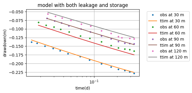
../_images/acd0f0dc379d79e7096cb9c6a070eb921878fdf0951a067e7b8c357c2dbb4e21.png

It is very difficult to find one set of optimal parameters. Different optimal parameters are found for different initial values.

Step 9. Analysis and summary of values simulated by different models#

Here we compare the simulations done with TTim with other software and the values reported in Kruseman and de Ridder (1970). The published values were determined by graphical adjustment to the Hantush family of type curves (Hantush, 1955). To compare the results reported in the literature with different models, we begin by analysing the values obtained without storage. Alongside with TTim and literature values, we report the values MLU (Carlson & Randall, 2012) and AQTESOLV (Duffield, 2007) models, reported by Xinzhu (2020)

Step 9.1. Comparison of results of models without storage#

t1 = pd.DataFrame(
    columns=["k [m/d]", "Ss [1/m]", "c [d]", "Sll [1/m]"],
    index=[
        "Hantush",
        "ttim - semi-confined",
        "MLU",
        "AQTESOLV",
    ],
)
t1.loc["Hantush"] = [45.332, 4.762e-5, 331.141, "-"]
t1.loc["ttim - semi-confined"] = np.append(c0.parameters["optimal"].values, "-")
t1.loc["MLU"] = [45.186, 3.941e-05, 769.200, 3.611e-04]
t1.loc["AQTESOLV"] = [49.286, 4.559e-05, 745.156, "-"]
rmse = [0.005917, c0.rmse(), 0.005941, 0.007245]
t1["RMSE [m]"] = rmse
t1

	k [m/d]	Ss [1/m]	c [d]	Sll [1/m]	RMSE [m]
Hantush	45.332	0.000048	331.141	-	0.005917
ttim - semi-confined	45.332094878897756	4.762233005640743e-05	331.1797887880521	-	0.005917
MLU	45.186	0.000039	769.2	0.000361	0.005941
AQTESOLV	49.286	0.000046	745.156	-	0.007245

Step 9.2. Comparison of results of models with storage#

t2 = pd.DataFrame(
    columns=["k [m/d]", "Ss [1/m]", "c [d]", "Sll [1/m]"],
    index=["ttim - semi-confined", "MLU", "AQTESOLV"],
)
t2.loc["MLU"] = [45.335, 4.668e-05, 331.400, 1.284e-05]
t2.loc["AQTESOLV"] = [45.159, 4.100e-05, 367.577, 2.868e-05]
t2.loc["ttim - semi-confined"] = c1.parameters["optimal"].values
t2["RMSE [m]"] = [c1.rmse(), 0.004941, 0.005861]
t2

	k [m/d]	Ss [1/m]	c [d]	Sll [1/m]	RMSE [m]
ttim - semi-confined	44.398308	0.00004	885.737117	0.000531	0.005923
MLU	45.335	0.000047	331.4	0.000013	0.004941
AQTESOLV	45.159	0.000041	367.577	0.000029	0.005861

Overall, all models found similar K values for the aquifer. TTim models differed significantly from the MLU and AQTESOLV solutions for the aquitard storage and resistance.

References#

Bakker, M. Semi-analytic modeling of transient multi-layer flow with TTim. Hydrogeol J 21, 935–943 (2013). https://doi.org/10.1007/s10040-013-0975-2
Carlson F, Randall J (2012) MLU: a Windows application for the analysis of aquifer tests and the design of well fields in layered systems. Ground Water 50(4):504–510
Duffield, G.M., 2007. AQTESOLV for Windows Version 4.5 User’s Guide, HydroSOLVE, Inc., Reston, VA.
Newville, M.,Stensitzki, T., Allen, D.B., Ingargiola, A. (2014) LMFIT: Non Linear Least-Squares Minimization and Curve Fitting for Python.https://dx.doi.org/10.5281/zenodo.11813. https://lmfit.github.io/lmfit-py/intro.html (last access: August,2021).
Yang, Xinzhu (2020) Application and comparison of different methodsfor aquifer test analysis using TTim. Master Thesis, Delft University of Technology (TUDelft), Delft, The Netherlands.