3. Slug Test - Multi-well in confined aquifer#

This test is taken from examples of AQTESOLV.

Step 1. Import required libraries#

import matplotlib.pyplot as plt
import numpy as np
import pandas as pd

import ttim as ttm

plt.rcParams["figure.figsize"] = [5, 3]

Introduction and Conceptual Model#

In this notebook, we reproduce the work of Yang (2020) to check the TTim performance in analysing slug-test. We later compare the solution in TTim with the KGS analytical model (Hyder et al. 1994) implemented in AQTESOLV (Duffield, 2007) and to the MLU model (Carlson & Randall, 2012).

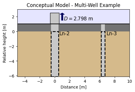
This Slug Test was reported in Butler (1998). A well (Ln-2) fully penetrates a sandy confined aquifer, with 6.1 m thickness. Additionally, a fully penetrating observation well (Ln-3) is placed 6.45 m away from the test well.

The slug displacement is 2.798 m. Head change was recorded at the slug well and the observation well. The well and casing radii of the slug well are 0.102 and 0.051 m, respectively. For the observation well, they are 0.051 and 0.025 m, respectively.

The conceptual model can be seen in the figure below.

Show code cell source

Hide code cell source

import matplotlib.pyplot as plt

##Now printing the conceptual model figure:

fig = plt.figure()
ax = fig.add_subplot(1, 1, 1)
# sky
sky = plt.Rectangle((-5, 1), width=15, height=3, fc="b", zorder=0, alpha=0.1)
ax.add_patch(sky)

# Aquifer:
ground = plt.Rectangle(
    (-5, -6.1),
    width=15,
    height=6.1,
    fc=np.array([209, 179, 127]) / 255,
    zorder=0,
    alpha=0.9,
)
ax.add_patch(ground)

well = plt.Rectangle(
    (-0.5, -(6.1)), width=1, height=(7.1), fc=np.array([200, 200, 200]) / 255, zorder=1
)
ax.add_patch(well)

# Confining Unit
conf = plt.Rectangle(
    (-5, 0), width=15, height=1, fc=np.array([100, 100, 100]) / 255, zorder=0, alpha=0.9
)
ax.add_patch(conf)

# Wellhead
wellhead = plt.Rectangle(
    (-0.6, 1),
    width=1.2,
    height=1.5,
    fc=np.array([200, 200, 200]) / 255,
    zorder=2,
    ec="k",
)
ax.add_patch(wellhead)

# Screen for the well:
screen = plt.Rectangle(
    (-0.5, -(6.1)),
    width=1,
    height=6.1,
    fc=np.array([200, 200, 200]) / 255,
    alpha=1,
    zorder=2,
    ec="k",
    ls="--",
)
screen.set_linewidth(2)
ax.add_patch(screen)
pumping_arrow = plt.Arrow(x=1, y=1.5, dx=0, dy=1, color="#00035b")
ax.add_patch(pumping_arrow)
ax.text(x=1.2, y=1.5, s=r"$ D = 2.798$ m", fontsize="large")

# Piezometer
piez = plt.Rectangle(
    (6.20, -(6.1)),
    width=0.5,
    height=(7.1),
    fc=np.array([200, 200, 200]) / 255,
    zorder=1,
)
ax.add_patch(piez)
screen_piez = plt.Rectangle(
    (6.2, -(6.1)),
    width=0.5,
    height=6.1,
    fc=np.array([200, 200, 200]) / 255,
    alpha=1,
    zorder=2,
    ec="k",
    ls="--",
)
screen_piez.set_linewidth(2)
ax.add_patch(screen_piez)

# last line
line = plt.Line2D(xdata=[-200, 1200], ydata=[1, 1], color="k")
ax.add_line(line)

# Water table
# wt = plt.Line2D(xdata= [-200,1200], ydata = [0,0], color = "b")
# ax.add_line(wt)

ax.text(0.6, -0.5, s="Ln-2", fontsize="large")
ax.text(6.9, -0.5, "Ln-3", fontsize="large")
ax.set_xlim([-5, 10])
ax.set_ylim([-6.1, 3])
ax.set_xlabel("Distance [m]")
ax.set_ylabel("Relative height [m]")
ax.set_title("Conceptual Model - Multi-Well Example");

../_images/c0c95f39d42a0c6398aa75d6003af865beee76962a60ce9a086611099546a1ff.png

Step 2. Set basic parameters#

H0 = 2.798  # initial displacement, m
b = -6.1  # aquifer thickness, m
rw1 = 0.102  # well radius of Ln-2 Well, m
rw2 = 0.071  # well radius of observation Ln-3 Well, m
rc1 = 0.051  # casing radius of Ln-2 Well, m
rc2 = 0.025  # casing radius of Ln-3 Well, m
r = 6.45  # distance from observation well to test well, m

Step 3. Converting slug displacement to volume#

Q = np.pi * rc1**2 * H0
print("Slug:", round(Q, 5), "m^3")

Slug: 0.02286 m^3

Step 4. Load data#

data1 = np.loadtxt("data/ln-2.txt")
t1 = data1[:, 0] / 60 / 60 / 24  # convert time from seconds to days
h1 = data1[:, 1]
data2 = np.loadtxt("data/ln-3.txt")
t2 = data2[:, 0] / 60 / 60 / 24
h2 = data2[:, 1]

Step 5. Create First Model - single layer#

We begin with a single layer model built in ModelMaq. Details on setting up the model can be seen in: Confined 1 - Oude Korendijk.

The slug well is set accordingly. Details on setting up the Well object can be seen in: Slug 1 - Pratt County.

ml_0 = ttm.ModelMaq(kaq=10, z=[0, b], Saq=1e-4, tmin=1e-5, tmax=0.01)
w_0 = ttm.Well(
    ml_0, xw=0, yw=0, rw=rw1, rc=rc1, tsandQ=[(0, -Q)], layers=0, wbstype="slug"
)
ml_0.solve()

self.neq  1
solution complete

Step 6. Model calibration both simultaneous wells#

The procedures for calibration can be seen in Unconfined 1 - Vennebulten

We calibrate hydraulic conductivity and specific storage, as in the KGS model (Hyder et al. 1994).

# unknown parameters: kaq, Saq
ca_0 = ttm.Calibrate(ml_0)
ca_0.set_parameter(name="kaq0", initial=10)
ca_0.set_parameter(name="Saq0", initial=1e-4)
ca_0.seriesinwell(name="Ln-2", element=w_0, t=t1, h=h1)
ca_0.series(name="Ln-3", x=r, y=0, layer=0, t=t2, h=h2)
ca_0.fit()

....................................
Fit succeeded.

/tmp/ipykernel_1356/3825640883.py:3: DeprecationWarning: Setting layers in the parameter name is deprecated. Set the layers= keyword argument for parameter 'kaq0' to silence this warning. The parameter name can still include layer info, but this will be ignored in a future version of TTim.
  ca_0.set_parameter(name="kaq0", initial=10)
/tmp/ipykernel_1356/3825640883.py:4: DeprecationWarning: Setting layers in the parameter name is deprecated. Set the layers= keyword argument for parameter 'Saq0' to silence this warning. The parameter name can still include layer info, but this will be ignored in a future version of TTim.
  ca_0.set_parameter(name="Saq0", initial=1e-4)

display(ca_0.parameters)
print("RMSE:", ca_0.rmse())

	layers	optimal	std	perc_std	pmin	pmax	initial	inhoms	parray
kaq0_0_0	None	1.166114	2.926073e-03	0.250925	-inf	inf	10.0000	None	[[1.1661141715204393]]
Saq0_0_0	None	0.000009	1.158398e-07	1.234728	-inf	inf	0.0001	None	[[9.381812725641323e-06]]

RMSE: 0.010236347641794178

hm1_0 = w_0.headinside(t1)
hm2_0 = ml_0.head(r, 0, t2, layers=0)
plt.semilogx(t1, h1 / H0, ".", label="obs ln-2")
plt.semilogx(t1, hm1_0[0] / H0, label="ttim ln-2")
plt.semilogx(t2, h2 / H0, ".", label="obs ln-3")
plt.semilogx(t2, hm2_0[0] / H0, label="ttim ln-3")
plt.xlabel("time [d]")
plt.ylabel("Normalized Head: h/H0")
plt.title("Model Results - Single layer model")
plt.legend()
plt.grid()

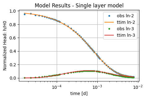
../_images/17f566d0a7fe38a2fc1010e6d249efb9da68c5df9649c5edd59ec0b6dc249182.png

In general, the single-layer model seems to be performing well, with a good visual fit between observations and the model.

Step 8. Calibration with well skin resistance#

Now we test if the skin resistance of the well has an impact on model calibration. Therefore, we add the res parameter in the calibration settings. We use the one-layer model.

# unknown parameters: kaq, Saq, res
ca_1 = ttm.Calibrate(ml_0)
ca_1.set_parameter(name="kaq0", initial=10)
ca_1.set_parameter(name="Saq0", initial=1e-4)
ca_1.set_parameter_by_reference(name="res", parameter=w_0.res, initial=0)
ca_1.seriesinwell(name="Ln-2", element=w_0, t=t1, h=h1)
ca_1.series(name="Ln-3", x=r, y=0, layer=0, t=t2, h=h2)
ca_1.fit(report=True)

...
...
............................................
..
..
........
Fit succeeded.
[[Fit Statistics]]
    # fitting method   = leastsq
    # function evals   = 59
    # data points      = 162
    # variables        = 3
    chi-square         = 0.01256036
    reduced chi-square = 7.8996e-05
    Akaike info crit   = -1527.29854
    Bayesian info crit = -1518.03575
[[Variables]]
    kaq0_0_0:  1.24195060 +/- 0.01093488 (0.88%) (init = 10)
    Saq0_0_0:  9.0454e-06 +/- 1.0984e-07 (1.21%) (init = 0.0001)
    res:       0.02259652 +/- 0.00297201 (13.15%) (init = 0)
[[Correlations]] (unreported correlations are < 0.100)
    C(kaq0_0_0, res)      = +0.9660
    C(kaq0_0_0, Saq0_0_0) = -0.5094
    C(Saq0_0_0, res)      = -0.4050

/tmp/ipykernel_1356/2310785823.py:3: DeprecationWarning: Setting layers in the parameter name is deprecated. Set the layers= keyword argument for parameter 'kaq0' to silence this warning. The parameter name can still include layer info, but this will be ignored in a future version of TTim.
  ca_1.set_parameter(name="kaq0", initial=10)
/tmp/ipykernel_1356/2310785823.py:4: DeprecationWarning: Setting layers in the parameter name is deprecated. Set the layers= keyword argument for parameter 'Saq0' to silence this warning. The parameter name can still include layer info, but this will be ignored in a future version of TTim.
  ca_1.set_parameter(name="Saq0", initial=1e-4)

display(ca_1.parameters)
print("RMSE:", ca_1.rmse())

	layers	optimal	std	perc_std	pmin	pmax	initial	inhoms	parray
kaq0_0_0	None	1.241951	1.093488e-02	0.880460	-inf	inf	10.0000	None	[[1.2419506031765226]]
Saq0_0_0	None	0.000009	1.098350e-07	1.214268	-inf	inf	0.0001	None	[[9.045371453736228e-06]]
res	NaN	0.022597	2.972009e-03	13.152507	-inf	inf	0.0000	NaN	[[0.02259651858545118]]

RMSE: 0.00880528748763316

hm1_1 = w_0.headinside(t1)
hm2_1 = ml_0.head(r, 0, t2, layers=0)
plt.semilogx(t1, h1 / H0, ".", label="obs ln-2")
plt.semilogx(t1, hm1_1[0] / H0, label="ttim ln-2")
plt.semilogx(t2, h2 / H0, ".", label="obs ln-3")
plt.semilogx(t2, hm2_1[0] / H0, label="ttim ln-3")
plt.xlabel("time [d]")
plt.ylabel("Normalized Head: h/H0")
plt.title("Model Results - Single layer model with res")
plt.legend()
plt.grid()

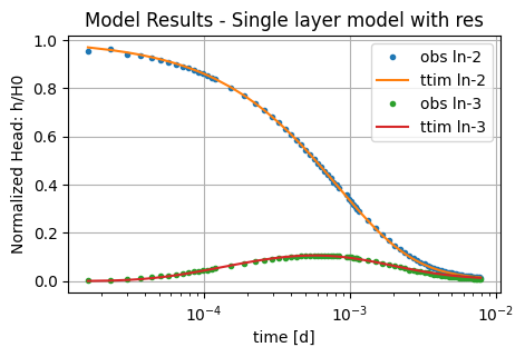
../_images/f78a36abb85fc6e8ae550ac0ba3e9f44612092abec43fd15420d7cf58ee4ef78.png

Adding well screen resistance does not improve the performance significantly, while the AIC value increases. Thus, it is recommended to leave it out of the model.

Step 11. Analysis and comparison of simulated values#

We now compare the values in TTim and also add the results of the modelling done in AQTESOLV and MLU by Yang (2020).

ta = pd.DataFrame(
    columns=["k [m/d]", "Ss [1/m]"],
    index=["MLU", "AQTESOLV", "ttim", "ttim_skin"],
)
ta.loc["AQTESOLV"] = [1.166, 9.368e-06]
ta.loc["MLU"] = [1.311, 8.197e-06]
ta.loc["ttim"] = ca_0.parameters["optimal"].values
ta.loc["ttim_skin"] = ca_0.parameters["optimal"].values[:2]
ta["RMSE [m]"] = [0.010373, 0.009151, ca_0.rmse(), ca_1.rmse()]
ta.style.set_caption("Comparison of parameter values and error under different models")

Comparison of parameter values and error under different models
	k [m/d]	Ss [1/m]	RMSE [m]
MLU	1.311000	0.000008	0.010373
AQTESOLV	1.166000	0.000009	0.009151
ttim	1.166114	0.000009	0.023000
ttim_skin	1.166114	0.000009	0.008805

The parameters in every model closely match each other. The error was also very similar.

References#

Butler, J.J., Jr., 1998. The Design, Performance, and Analysis of Slug Tests, Lewis Publishers, Boca Raton, Florida, 252p.
Hyder, Z., Butler Jr, J.J., McElwee, C.D., Liu, W., 1994. Slug tests in partially penetrating wells. Water Resources Research 30, 2945–2957.
Duffield, G.M., 2007. AQTESOLV for Windows Version 4.5 User’s Guide, HydroSOLVE, Inc., Reston, VA.
Yang, Xinzhu (2020) Application and comparison of different methodsfor aquifer test analysis using TTim. Master Thesis, Delft University of Technology (TUDelft), Delft, The Netherlands.